U
N
I V
E R S I T
A
S
S
A
R
A V I E N
S
I
S
Reduction of
Acyclic Phase-Type Representations
Dissertation zur Erlangung des Grades des Doktors der Ingenieurwissenschaften der Naturwissenschaftlich-Technischen Fakultäten der Universität des Saarlandes
Muhammad Reza Pulungan
Tag des Kolloquiums 27.05.2009
Dekan Prof. Dr. Joachim Weickert
Prüfungsausschuss
Vorsitzender Prof. Dr. Dr. h.c. mult. Reinhard Wilhelm Berichterstattende Prof. Dr.-Ing. Holger Hermanns
Abstract
Acyclic phase-type distributions are phase-type distributions with triangular matrix representations. They constitute a versatile modelling tool, since they (1) can serve as approximations to any continuous probability distribution, and (2) exhibit special properties and characteristics that usually make their analysis easier. The size of the matrix representations has a strong effect on the computational efforts needed in an-alyzing these distributions. These representations, however, are not unique, and two representations of the same distribution can differ drastically in size.
This thesis proposes an effective algorithm to reduce the size of the matrix represen-tations without altering their associated distributions. The algorithm produces signifi-cantly better reductions than existing methods. Furthermore, the algorithm consists in only standard numerical computations, and therefore is straightforward to implement. We identify three operations on acyclic phase-type representations that arise often in stochastic models. Around these operations we develop a simple stochastic process calculus, which provides a framework for stochastic modelling and analysis. We prove that the representations produced by the three operations are “almost surely” minimal, and the reduction algorithm can be used to obtain these almost surely minimal rep-resentations. The applicability of these contributions is exhibited on a variety of case studies.
Zusammenfassung
Azyklische Phasentypverteilungen sind Phasentypverteilungen, deren Matrixdarstel-lung eine Dreiecksmatrix ist. Sie stellen ein vielseitiges Modellierungswerkzeug dar, da sie einerseits als Approximationen jeder beliebigen kontinuierlichen Wahrscheinlich-keitsverteilung dienen können, und andererseits spezielle Eigenschaften und Charak-teristiken aufweisen, die ihre Analyse vereinfachen. Die Größe der Matrixdarstellung hat dabei einen starken Einfluss auf den Berechnungsaufwand, der zur Analyse solcher Verteilungen nötig ist. Die Matrixdarstellung ist jedoch nicht eindeutig, und zwei ver-schiedene Darstellungen ein und derselben Verteilung können sich drastisch in ihrer Größe unterscheiden.
In dieser Arbeit wird ein effektiver Algorithmus zur Verkleinerung der Matrixdar-stellung vorgeschlagen, der die mit der DarMatrixdar-stellung assoziierte Verteilung nicht verän-dert. Dieser Algorithmus verkleinert die Matrizen dabei beträchtlich stärker als bereits existierende Methoden. Darüberhinaus bedient er sich nur numerischer Standard-verfahren, wodurch er einfach zu implementieren ist. Wir identifizieren drei Opera-tionen auf azyklischen Phasentypdarstellung, die in stochastischen Modellen häufig anzutreffen sind. Von diesen Operationen ausgehend entwickeln wir einen einfachen stochastischen Prozess-Kalkül, der eine grundlegende Struktur für stochastische Mo-dellierung und Analyse darstellt. Wir zeigen, dass die durch die drei Operationen erzeugten Darstellungen „beinahe gewiss“ minimal sind und dass der Reduktionsal-gorithmus benutzt werden kann, um diese beinahe gewiss minimalen Darstellungen zu erzeugen. Die Anwendbarkeit dieser Beiträge wird an einer Reihe von Fallstudien exemplifiziert.
Acknowledgements
First and foremost, I thank my supervisor Holger Hermanns for his patience and dili-gence in guiding me throughout my years in Saarbrücken. He has been an excellent mentor who is ever ready for discussions.
I would also like to thank my colleagues in the group: Pepijn Crouzen, Christian Eisentraut, Moritz Hahn, David Jansen, Sven Johr, Christa Schäfer and Lijun Zhang, for their friendship and support.
Special thanks go to Basileios Anastasatos, Pepijn Crouzen and Christian Eisentraut for helping me proofreading this thesis. In the end, however, mistakes are mine alone.
I am lucky to have a big and happy family. I am grateful to my mother; my sisters: Nevi and Elvida; my brothers: Fauzi, Lian, Randi and Yazid; for their endless love and support.
This thesis is dedicated to the memory of my father.
Contents
1 Introduction
12 Preliminaries
52.1 Mathematical Notations . . . 6
2.2 Random Variables . . . 6
2.3 Exponential Distributions . . . 7
2.4 Markov Chains . . . 7
2.4.1 Stochastic Processes . . . 7
2.4.2 Markov Processes . . . 8
2.4.3 Discrete-Time Markov Chains . . . 8
2.4.4 Continuous-Time Markov Chains . . . 11
2.5 Phase-Type Distributions . . . 13
2.5.1 General Notions and Concepts . . . 16
2.5.2 Order and Degree . . . 18
2.5.3 Dual Representations . . . 19
2.5.4 Characterization . . . 20
2.5.5 Closure Properties . . . 21
2.6 Acyclic Phase-Type Distributions . . . 23
2.6.1 Characterization . . . 24
2.6.2 Closure Properties . . . 25
2.6.3 Erlang and Hypoexponential Distributions . . . 25
2.7 The Polytope of Phase-Type Distributions . . . 26
2.7.1 Residual-Life Operator . . . 27
2.7.2 Simplicity and Majorization . . . 28
2.7.3 Geometrical View of APH Representations . . . 30
2.8 Matrix-Exponential Distributions . . . 33
3 Reducing APH Representations
35 3.1 Acyclic Canonical Forms . . . 363.1.1 Ordered Bidiagonal Representation . . . 37
3.1.2 Cox Representation . . . 38
3.2 Transformation to Ordered Bidiagonal . . . 39
3.3 Transformation Algorithms . . . 41
3.3.1 Cumani’s Algorithm . . . 41
3.3.2 O’Cinneide’s Algorithm . . . 42
3.3.3 Spectral Polynomial Algorithm . . . 43
xii CONTENTS
3.4 Reducing the Representations . . . 44
3.4.1 TheL-terms . . . 44
3.4.2 Reduction . . . 45
3.4.3 Algorithm . . . 48
3.5 Examples: Fault-Tolerant System . . . 50
3.6 Relation to Lumping . . . 51
3.7 Conclusion . . . 56
4 Operations on Erlang Distributions
59 4.1 Refining the Basic Series . . . 604.2 Convolution Operation . . . 63
4.3 Minimum Operation . . . 64
4.3.1 The Minimum of Two Erlang Distributions . . . 64
4.3.2 The Minimum of More Erlang Distributions . . . 65
4.3.3 The Minimal of the Minimum . . . 67
4.4 Maximum Operation . . . 69
4.4.1 The Maximum of Two Erlang Distributions . . . 70
4.4.2 The Maximum of More Erlang Distributions . . . 71
4.4.3 The Minimal of the Maximum . . . 73
4.5 Conclusion . . . 76
5 The Use of APH Reduction
79 5.1 Minimal and Non-Minimal Representations . . . 805.2 When Order = Algebraic Degree . . . 82
5.2.1 Known Results . . . 82
5.2.2 Our Reduction Algorithm . . . 86
5.3 Operations on APH Representations . . . 90
5.3.1 Convolution Operation . . . 90
5.3.2 Minimum and Maximum Operations . . . 93
5.4 Almost Surely Minimal . . . 96
5.5 Conclusion . . . 99
6 A Simple Stochastic Calculus
101 6.1 CCC Processes . . . 1026.1.1 Intuitions . . . 102
6.1.2 Syntax . . . 104
6.1.3 Semantics . . . 105
6.2 CCC Processes and PH Distributions . . . 109
6.3 Some Notions of Equivalence . . . 112
6.3.1 Bisimulations . . . 112
6.3.2 PH-Equivalence . . . 114
6.4 Equivalence Checking and Process Reduction . . . 115
6.4.1 Algorithmic Considerations . . . 116
6.4.2 Compositional Considerations . . . 117
CONTENTS xiii
7 Case Studies
1197.1 Fault Trees with PH Distributions . . . 120
7.2 Fault-Tolerant Parallel Processors . . . 123
7.3 Delay in a Railway Network . . . 127
7.4 Conclusion . . . 138
8 Conclusion
141Appendices
A Basic Concepts
143 A.1 Poisson Processes . . . 143A.2 Kronecker Product and Sum . . . 144
A.3 Some Concepts from Convex Analysis . . . 144
A.3.1 Affine Sets . . . 144
A.3.2 Convex Sets . . . 145
B Proofs
147 B.1 Lemma 3.14 . . . 147B.2 Lemma 5.14 . . . 149
B.3 Lemma 6.12 . . . 150
B.4 Lemma 6.18 . . . 154
Chapter 1
Introduction
Due to the incomplete nature of our knowledge of the physical systems we interact with, they appear to exhibit stochastic behaviors. This is also true for most of com-puter and electronic communication systems we increasingly rely on. These stochastic behaviors usually influence the performance of a system, but they may also affect the functional characteristics or even the correctness of the system. When such systems are analyzed, it is important therefore not to neglect their stochastic behaviors.
One of the many approaches we can take in analyzing such systems ismodel-based analysis. In this approach, the analysis is directed at an abstract description of the system—its components and their interactions as well as the system’s interactions with the environment—instead of at the system itself [Hav98]. In many cases, this approach is taken because access to the real system is difficult or impossible. But more importantly, this approach allows us to abstract from the real system, to focus and con-centrate on the parts of the system that are relevant and interesting. This way, analysis can be greatly simplified.
Further, one of the ways to carry out a model-based analysis isstate-based analysis. A state-based analysis proceeds by modelling the system in terms of its states (i.e., some distinguishable characteristics) and how the system changes from one state to others. An obvious requirement in this analysis is that the possible states to which the system changes from a particular state must be a well-defined subset of the state space. In this field, Markov chains play a befitting role: since the immediate future state of a Markov chain depends only on its current state and not on the states visited prior to the current one, they meet the requirement.
Research in the field of stochastic state-based analysis has been flourishing for many years. Progress has been made in the foundation and algorithms for model checking Markov models, especially in the continuous-time setting [ASSB00, BHHK03]. Various Markovian process calculi, such as MTIPP [HR94], PEPA [Hil96], EMPA [BG96] and IMC [Her02], have been proposed, which open the possibility of compositionality in the construction of models. The field also enjoys a proliferation of tools, such as PRISM[HKNP06],ETMCC[HKMKS03], its successorMRMC[KKZ05] and CASPA[RSS08].
A comparative study of some of these prominent tools can be found in [JKO+08].
Markovian modelling and analysis are widely used in diverse fields of computer science and engineering, from queueing theory [Neu81, Asm92], computer network design [CR91, KSH03], to reliability analysis [CKU92], for instance in the analysis of dynamic fault trees [MDCS98, BCS07a].
However, the field of stochastic state-based analysis is faced by a major challenge:
2 Chapter 1. Introduction
the state-space explosion problem. Compositions of Markov models are usually accom-plished by the cross products of the state spaces of the involved models. As a result, the state space of composite models grows too big very quickly, they exceed the size of the memory of standard modern computers. One of the ways to deal with this challenge is to avoid representing and working with explicit states, but instead to encode the state space in a symbolic and more compact way, for instance by using binary decision diagrams (BDDs) [HKN+03] or Kronecker representations [PA91, BCDK00, HK01].
Another way to deal with the challenge is by using lumping [KS76, Nic89, Buc94]. Lumping defines an aggregation of a Markov chain by identifying a partitioning of its state space such that all states in a particular partition share some common charac-teristics. When such partitioning can be identified, all states that belong to a single partition can be aggregated by (or lumped together into) a single state without altering the overall stochastic behavior of the original Markov chain. Several methods exist to identify the partitioning; the most widely used among them are those based on bisim-ulation equivalences on Markov chains [Bra02, DHS03]. More recently, improvements on the bisimulation-based lumping algorithm especially tailored for models without cycles are provided in [CHZ08].
A question, nevertheless, arises: is bisimulation-based lumping useful in practice? The answer is affirmative as shown by the authors of [KKZJ07]. They showed that the time needed to analyze a Markov chainmostly exceedsthe combination of the time needed to aggregate it and the time needed to analyze the aggregated Markov chain. Their results also indicate that enormous state-space reductions (up to logarithmic savings) may be obtained through lumping. As it stands nowadays, lumping is the best mechanism we have to reduce the size of the state space of Markov models.
This thesis proposes a reduction algorithm that goes beyond lumping, in the sense that, the new algorithm is guaranteed to reduce the state space of Markov models no less than lumping. The algorithm performs state-space reduction of representations of (continuous-time) phase-type distributions.
Phase-type distributions are a versatile and tractable class of probability distribu-tions, retaining the principal analytical tractability of exponential distribudistribu-tions, on which they are based. Phase-type distributions are topologically dense [JT88] on the support set[0,∞). Therefore, they can be used to approximate arbitrarily closely other probability distributions or traces of empirical distributions obtained from experimen-tal observations. This broadens the applicability of stochastic analysis of this type, since we can then incorporate in our models probability distributions that would be otherwise intractable by fitting phase-type distributions to them.
Any phase-type distribution agrees with the distribution of the time until absorp-tion in some (continuous-time) Markov chain with an absorbing state [Neu81]. Such a Markov chain is actually the basis of numerical or analytical analysis for models in-volving that phase-type distribution, and it is therefore called therepresentationof that distribution. These representations are not unique: distinct absorbing Markov chains may represent the same distribution, and any phase-type distribution is represented by infinitely many distinct absorbing Markov chains. The representations differ in par-ticular with respect to theirsize,i.e., the number of their states and transitions. Thus, for a given phase-type distribution, an obvious question to pose is what theminimal
3
The problem of identifying and constructing smaller-sized representations is one of the most interesting theoretical research questions in the field of phase-type dis-tributions. The focus of this thesis is on the class of acyclic phase-type distributions,
i.e., phase-type distributions with (upper) triangular matrix representations. Like the general phase-type distributions, acyclic phase-type distributions are also topologically dense on the support set[0,∞)[JT88].
The systematic study of acyclic phase-type representations was initiated in [Cum82], and later, in [O’C91, O’C93], minimality conditions are identified, but without algorith-mic considerations. A closed-form solution for the transient analysis of acyclic Markov chains—hence also acyclic phase-type representations—is presented in [MRT87]. The quest for an algorithm to construct the minimal representation of any acyclic phase-type distribution has recently seen considerable advances: an algorithm for comput-ing minimal representations of acyclic phase-type distributions is provided in [HZ07a]. This algorithm involves converting a given acyclic phase-type distribution to a repre-sentation that only contains states representing the poles of the distribution. This representation does not necessarily represent an acyclic phase-type distribution, but a matrix-exponential distribution [Fac03]. If this is the case, another state and its to-tal outgoing rate are determined and added to the representation. This is performed one by one until an acyclic phase-type representation is obtained. This results in a representation of provably minimal size. This algorithm involves solving a system of non-linear equations for each additional state.
Our Contribution The algorithm developed in this thesis addresses the same problem, but in the opposite way. Instead of adding states to a representation until it becomes an acyclic phase-type representation, we eliminate states from the given representation as we proceed, until no further elimination is possible. An elimination of a state involves solving a system of linear equations. The reduction algorithm we propose is of cubic complexity in the size of the state space of the given representation, and only involves standard numerical computations. The algorithm is guaranteed to return a smaller or equal size representation than the given one, and also than the aggregated representation produced by lumping. This state-space reduction algorithm is the core contribution of this thesis, and it is embedded in a collection of observations of both fundamental and pragmatic nature.
We also identify three operations on acyclic phase-type distributions and represen-tations that arise often when constructing a stochastic model. These operations are convolution, minimum and maximum. Around these operations we develop a simple stochastic process calculus that captures the generation and manipulation of acyclic phase-type representations. This process calculus provides a framework for stochastic modelling and analysis. In this calculus, we analyze the reduction algorithm more deeply to identify the circumstances where it is beneficial to use it. We prove that representations produced by the three operations are “almost surely” minimal, and the reduction algorithm can be used to obtain these almost surely minimal represen-tations. On the more specific Erlang distributions, we show that the representations obtained from the application of each of these operations can always be reduced to minimal representations.
4 Chapter 1. Introduction
Organization of the Thesis The thesis is divided into eight chapters. They are organized as follows:
• Chapter 2 provides a comprehensive introduction to phase-type distributions, acyclic phase-type distributions and other basic concepts and notions required throughout the thesis. We do our best to include most of contemporary knowl-edge and results in the field of acyclic phase-type distributions in this chapter.
• In Chapter 3, we develop our reduction algorithm. We first set the ground by visiting several previous algorithms that form the basis of our algorithm. A small example is provided to guide the reader and to clarify the inner workings of the algorithm. We discuss the relation of the algorithm to weak-bisimulation-based lumping.
• Chapter 4 deals primarily with the minimal representations of the convolution, minimum and maximum of Erlang distributions. In proving minimalities, we put forward a new concept of the core series, which improves on a similar and existing concept, and furthermore provides a handy tool in many proofs.
• In Chapter 5, we delve more deeply into the reduction algorithm. We compare it with several existing results related to acyclic phase-type representations. We identify the conditions under which the algorithm is useful. We discuss the effect of the three operations on acyclic phase-type representations, and the role the algorithm plays in reducing the results of the operations.
• In Chapter 6, we develop a simple stochastic process calculus to generate and ma-nipulate acyclic phase-type representations. We define three congruent notions of equivalence on processes defined in this calculus.
• In Chapter 7, we demonstrate the applicability of the reduction algorithm by analyzing three case studies. From the case studies we learn the strength and the weakness of the algorithm.
Chapter 2
Preliminaries
This chapter lays out general concepts, notions and notations used throughout the thesis. It also provides a coherent introduction to phase-type distributions, acyclic phase-type distributions, and their representations.
Related Work Most of the material in this chapter is based on existing literature. Stan-dard textbooks, such as [Ste94, Hav98, LR99, Tij07, Ros07], are useful guidelines in the expositions of the topics related to stochastic processes and Markov chains. NEUTS’ monograph [Neu81] and O’CINNEIDE’s seminal paper [O’C90] are the major sources for the topic of phase-type distributions. The concept of dual representations was first discussed in [CC93], and later expanded in [CM02]. The characterization of phase-type distributions was proved in [O’C90], while that of acyclic phase-phase-type distributions was proved in [Cum82, O’C91]. The closure characterizations of phase-type distribu-tions and acyclic phase-type distribudistribu-tions were presented in [MO92] and [AL82], re-spectively. The idea of the polytope of phase-type distributions was first developed in [O’C90], while the notions of PH-simplicity and PH-majorization were developed
in [O’C89]. The main references for the section on the geometrical view of acyclic phase-type representations are [DL82] and [HZ06a]. The short discussion on matrix-exponential distributions is mainly based on [AO98, Fac03].
Structure The chapter is organized as follows: Several basic mathematical notations related to matrices and vectors are summarized in Section 2.1. Sections 2.2 and 2.3 give an overview on the basic concepts of random variables and exponential distribu-tions. These two sections provide the necessary foundation for discussing stochastic and Markov processes, especially Markov chains, which are described in Section 2.4. In Sections 2.5 and 2.6, the concepts of type distributions and acyclic phase-type distributions are introduced, covering their parameterization and structural defi-nitions, important properties, characterizations, and closures. In Section 2.7, we dis-cuss a geometrical method for studying phase-type distributions by examining their polytopes. Finally, Section 2.8 provides a brief introduction to matrix-exponential dis-tributions, touching only the notions that are relevant to the thesis.
6 Chapter 2. Preliminaries
2.1
Mathematical Notations
The set of real numbers is denoted byR, and the set of integers is denoted by Z. The nonnegative restriction of the sets R and Z is denoted by R≥0 and respectively Z≥0,
while the strictly positive restriction of the sets is denoted byR+ andZ+, respectively.
Vectors are written with an arrow over them, e.g.,~v. The dimension of a vector is the number of its components. Let the dimension of~v ben, then its i-th component, for 1 ≤ i ≤ n, is denoted by~vi. Vector~e is a vector whose components are all equal
to 1. Vector~0 is a vector whose components are all equal to 0. The dimension of~e
or~0should be clear from the context. Column and row vectors are indistinguishable notationally; the context should clarify the distinction. Vector~v⊤ is the transpose of
vector~v. A vector~v ∈Rn
≥0 is stochastic if~v~e= 1, and sub-stochastic if~v~e≤1.
Matrices are written in bold capital letters,e.g.,A. The dimension of a matrix with
mrows and n columns ismn. For square matrices, the dimension is shortened to just
minstead of mm. The component in the i-th row and the j-th column, for1 ≤i≤ m
and1≤ j ≤ n, is denoted by A(i, j). MatricesA⊤andA−1 are the transpose and the inverse of matrixA, respectively.
2.2
Random Variables
The basic concept in probability theory is probability space, namely a tuple(Ω,F,Pr), where:
• Ωis thesample space, a set containing all possible outcomes of an experiment,
• F is aσ-algebraon subsets ofΩcalledevents,i.e.,F ⊆2Ω satisfying
1. Ω∈ F,
2. ifA∈ F then so is the complement ofArelative toΩ,i.e.,Ac ∈ F, and
3. for every sequence ofAi ∈ F,i≥1, thenS∞i=1Ai ∈ F,
• Pris a probability measure, namely a functionPr :F →[0,1]that satisfies
1. Pr(Ω) = 1, and
2. for every sequence of pair-wise disjoint events Ai ∈ F, i ≥ 1, Pr is σ
-additive,i.e.,Pr(P∞i=1Ai) =P∞i=1Pr(Ai).
On the probability space, we can define a random variable, which can be contin-uous or discrete. In this thesis, we focus on the contincontin-uous (real-valued) random variables. LetR∞:=R∪ {+∞,−∞}.
Definition 2.1. Let(Ω,F,Pr) be a probability space. A (continuous) random variable
X over the probability space is a functionX : Ω →R∞ such that for allt∈R
{ω|X(ω)≤t} ∈ F.
The continuous random variable defined above is characterized by its distribution functionF :R→[0,1]given by
2.3. Exponential Distributions 7
To shorten the notation, we write Pr(X ≤ t) instead of Pr({ω | X(ω) ≤ t}). The random variable is also characterized by itsprobability density functionf : R → [0,1]
such that
F(t) =
Z t
0
f(x)dx.
For the given probability space, thesupportof the probability measurePris defined as the smallest subsetA∈ F ofΩsuch thatPr(Ac) = 0.
2.3
Exponential Distributions
The negative exponential distributions, which in this thesis will always be referred to simply as the exponential distributions, are continuous probability distributions. They are widely used in stochastic models, such as in the fields of performance analysis, dependability, and queueing theory. The exponential distributions are memoryless, which means that their distribution functions do not depend on the amount of time that has passed. This property makes them suitable for modelling the time between independent occurrences of events that occur at some constant rate. Random variables, such as the interarrival time of jobs to a file server or the service time of a server in a queueing network, are often modelled by exponential distributions [Tri02].
Definition 2.2. A random variable X is distributed according to an exponential
distri-butionwith rateλ∈R+ if its distribution function is given by
F(t) = Pr(X ≤t) =
1−e−λt, t ∈
R≥0,
0, otherwise. (2.1)
The probability density function of the exponential distribution is
f(t) =
λe−λt, t
∈R+,
0, otherwise.
An exponential distribution with rateλis denoted by Exp(λ).
2.4
Markov Chains
In this section, we introduce discrete-time and continuous-time Markov chains. In order to do that, we need first to provide the background and underlying concepts of stochastic processes and Markov processes.
2.4.1
Stochastic Processes
Astochastic processis a collection of random variables{Xt |t∈ T }that are indexed by
a parametert, which takes values from a setT (usually the time domain). The values that Xt assumes are called states, and the set of all possible states is called the state
space, denoted by S. Both setsS andT can be discrete or continuous.
At a particular time t ∈ T, the random variableXt may take different values. The
distribution function of the random variableXtatt ∈ T is
8 Chapter 2. Preliminaries
This is called the cumulative distribution function (cdf) of the random variable or the first-order distribution of the stochastic process {Xt | t ∈ T }. This function can be
extended to then-th joint distribution of the process
F(~x,~t) = Pr(X~t1 ≤~x1, . . . , X~tn ≤~xn},
where vectors~x and~tare of dimensionn,~xi ∈ S and~ti ∈ T, for 1≤i≤n.
A stochastic process where the state occupied at a certain time point does not depend on the state(s) being occupied at any other time point is anindependent process. Mathematically, an independent process is a stochastic process whosen-th order joint distribution satisfies
F(~x,~t) =
n
Y
i=1
F(~xi,~ti) = n
Y
i=1
Pr(X~ti ≤~xi).
A stochastic process can also be a dependent process, in which case some form of dependency exists among successive states.
2.4.2
Markov Processes
A stochastic process where a dependency exists only between two successive states is called aMarkov process. Such a dependence is called Markov dependence or first-order dependence.
Definition 2.3. A stochastic process{Xt|t∈ T }is aMarkov processif for allt0 < t1 <
· · ·< tn < tn+1, the distribution of the conditional probability ofXtn+1, given the values
ofXt0,· · ·, Xtn, depends only onXtn, i.e.,
Pr(Xtn+1 ≤xn+1 |Xt0 =x0, . . . , Xtn =xn) = Pr(Xtn+1 ≤xn+1 |Xtn =xn). (2.2)
Equation (2.2) expresses theMarkov property: that for any given time pointtn, the
future behavior—i.e., the values the random variableXtn+1can take—depends only on
the current state at time pointtn (Xtn).
A Markov process is time-homogeneousif it is invariant to time shifts. This means that the behavior of the process is independent of the time of observation. In this case, for anyt1 < t2, x1 andx2
Pr(Xt2 ≤x2 |Xt1 =x1) = Pr(Xt2−t1 ≤x2 |X0 =x1).
All Markov processes discussed in this thesis are time-homogeneous.
If the state spaceS of a Markov process is discrete, the Markov process is aMarkov chain. Two types of Markov chains can be identified: discrete-time and continuous-time Markov chains.
2.4.3
Discrete-Time Markov Chains
A discrete-time Markov chain (DTMC) is a stochastic process {Xt | t ∈ Z≥0} that has
a discrete state space S and a discrete index set T := Z≥0 and satisfies the Markov
property (which in this case can be written as)
2.4. Markov Chains 9
wherex0,· · · , xn, xn+1 ∈ S.
Without loss of generality, assume that the elements ofSrange over a subset of the natural numbers. We call the conditional probabilitiespi,j(n) := Pr(Xn+1 =j |Xn=i)
thetransition probabilities. They are the probabilities of making a transition from state
i∈ Sto statej ∈ S when time increases fromnton+ 1. In time-homogeneousDTMCs,
pi,j(n) is independent ofn, namely for all n, m∈ Z+,pi,j(n) = pi,j(m). The transition
probabilities for all statesi, j ∈ S can be represented by atransition probability matrix P, where
P(i, j) =pi,j(n).
A time-homogeneous DTMC is fully described by its initial probability vector ~p(0)—
where ~pi(0) gives the probability that the DTMC starts in state i—and its transition
probability matrixP.
Graphical Representation A DTMCcan be represented by a labelled directed graph. The vertices of the graph stand for the states of the DTMC, and the name of a state is
placed inside the vertex that represents the state. A transition is represented by an edge in the graph. The probability associated with a transition is placed near the edge representing the transition. An example of such graph is depicted in Figure 2.1.
0 1 2
0.5
0.5
0.25
0.2
0.75
0.6
0.2
Figure 2.1: A Discrete-Time Markov Chain
Example 2.4. Consider the DTMC depicted in Figure 2.1. There are three states in the
DTMC, named 0, 1 and 2. The DTMC also has seven transitions. These transitions are shown together with their probabilities, for instance, transition from state 0 to state 1
occurs with probability0.5. The transition probability matrix of the DTMC is
P=
0.5 0.5 0
0.25 0 0.75
0.2 0.6 0.2
.
Transient Analysis The purpose of transient analysis is to determine the probability with which aDTMC occupies a state after a given number of transitions have occurred.
This probability is called thetransient probabilityafter the given number of transitions. The transient probabilities of all states after n transitions (~p(n)) can be obtained by evaluating
~p(n) =~p(0)Pn, n∈Z≥0,
10 Chapter 2. Preliminaries
Example 2.5. We use theDTMC depicted in Figure 2.1. Let~p0(0) = 1and ~pi(0) = 0, for
i= 1,2. The transient probability vector of theDTMC after 3 transitions can be computed as follows
~p(3) =~p(0)P3 = [1,0,0]
0.5 0.5 0
0.25 0 0.75
0.2 0.6 0.2
3
= [0.325,0.4125,0.2625].
These transient probabilities describe the probabilities of being in some state after 3 transitions starting from state 0. For instance, after 3 transitions the DTMC will be
in state 2 with probability 0.2625. Transient probabilities after more transitions have occurred can be computed in a similar fashion. The transient probability vector after 15 and 25 transitions, for instance, is
~p(15) = [0.3111,0.35567,0.33323], and
~p(25) = [0.3111,0.35556,0.33333].
In the previous example, we can observe that after a certain number of transi-tions, the transient probabilities converge to a limiting stationary distribution. It is interesting to know whether the limiting probabilities can be obtained directly since for some measures of interest these probabilities may be sufficient. However, such limiting probabilities do not always exist for all DTMCs. The conditions under
which these probabilities exist—ergodicity—can be found in standard textbooks, such as [Ste94, LR99, Hav98, Ros07, Tij07].
Steady-State Analysis Steady-state analysis is used to determine the transient proba-bilities when the equilibrium—i.e., when the effect of the initial distribution has dis-appeared [Ste94]—has been reached. These probabilities are called the steady-state probabilities. If the limit~v= limn→∞~p(n)exists, the steady-state probabilities~v can be
obtained from the system of linear equations
~v=~v P, X
i∈S
~vi = 1, and 0≤~vi ≤1. (2.3)
If limn→∞~p(n) does not exist, for instance when the DTMC is periodic [Ste94], it
can be shown by the Cesàro-limit [Tij07, LR99] that the system of equations (2.3) still yields a unique solution. Therefore, it is safe to define the solution of the system of equations as the steady-state probabilities.
Example 2.6. We continue using the DTMC depicted in Figure 2.1 in this example. For
the givenDTMC, the steady-state probability vector is[14 45,
16 45,
1 3].
Steady-state probabilities can be interpreted as the probabilities of discovering that the DTMC is in some state after it has been running for a long time. They can also be interpreted as the fraction of time theDTMC spends in some state in the long run. Thus,
for the example, it can be said that after a long running time theDTMC will be in state2
2.4. Markov Chains 11
2.4.4
Continuous-Time Markov Chains
A continuous-time Markov chain(CTMC) is a stochastic process{Xt |t ∈R≥0}that has
a discrete state spaceS, a continuous index set T := R≥0, and satisfies the Markov
property (which in this case can be written as)
Pr(Xtn+1 =xn+1 |Xt0 =x0,· · · , Xtn =xn) = Pr(Xtn+1 =xn+1 |Xtn =xn),
for allt0 < t1 <· · ·< tn < tn+1 ∈ T.
While aDTMC is described by its transition probability matrix, aCTMC is described
by itsrate matrixR. With every pair of statesi, j ∈ S, we associate arate r(i, j), such that r(i, j) determines the delay and the probability of the transition from state i to statej. The rates of the transitions between all pairs of states can then be conveniently represented byR, where
R(i, j) =r(i, j).
for alli, j ∈ S. Let the sum of the rates of all outgoing transitions from stateibeE(i),
i.e.,E(i) =Pj∈SR(i, j). We call this sum thetotal outgoing rateor therate of residence
of the state.
The semantics of the CTMC is as follows: at any given time point, the CTMC is in
one of the states. Let theCTMC enter state iat some time point. From this state, the CTMC can transition to any statej ∈ S ifR(i, j)>0. Assuming that the only outgoing transition from stateiis to statej, then the delay of this transition is governed by an exponential distribution with rateR(i, j), whose distribution function is
Fi,j(t) = 1−e−R(i,j)t.
However, when other outgoing transitions exist from statei, this delay must com-pete with the delays of the other transitions. Arace conditionoccurs among the delays, and the shortest among them wins. This shortest delay corresponds to the minimum of exponential distributions governing the delays of all outgoing transitions, which itself is an exponential distribution with ratePj∈SR(i, j), whose distribution function is
Fi(t) = 1−e−
P
j∈SR(i,j)t= 1−e−E(i)t.
This distribution describes the residence time in state i, namely the time the CTMC
resides there before making any transition. The probability that a particular transition to state j occurs (thus, its corresponding delay wins the race) given other transitions from stateiis
p(i, j) = PR(i, j)
k∈SR(i, k)
= R(i, j)
E(i) .
Hence, the probability of making a transition from state i to a state j within t time units is given byp(i, j)Fi(t) =p(i, j)(1−e−E(i)t).
A CTMC is completely specified by its initial probability vector ~p(0) and its rate
matrix R. Besides its rate matrixR, a CTMC can also be specified by its infinitesimal generator matrixQ, where
Q(i, j) =
R(i, j), i6=j,
12 Chapter 2. Preliminaries
Transient Analysis The transient probabilities (~p(t)) of a CTMC with initial probability
vector ~p(0) and rate matrix Q can be obtained by solving the system of differential equations
d
dt~p(t) =~p(t)Q. (2.4)
The solution of the system of equation is
~p(t) =~p(0)eQt. (2.5)
One of the ways to evaluate Equation (2.5) is by computing the matrix exponential directly. Several methods for computing matrix exponentials are available [ML03, ML78]. However, most of them suffer from numerical instabilities.
A numerically stable method for evaluating Equation (2.5) is the uniformization
or randomization method [Jen53, GM84, Gra91]. Using this method, the transient analysis of theCTMC proceeds by analyzing its uniformizedCTMC. A uniformizedCTMC
can be obtained by (1) choosing a rate Λ ≥ maxi∈SE(i), and then (2) uniformizing
the rate of residence of all states withΛ, namely by settingQ(i, i) = −Λ, for alli∈ S. The original and the uniformizedCTMCs are stochastically equivalent [BKHW05].
Now that all states have the same total outgoing rate, the residence times in all states have the same distribution. The only distinguishing feature of all states now is their transition probabilities
P=I+ Q
Λ,
whereIis the identity matrix. MatrixPtogether with the initial probability vector~p(0)
describe theembeddedDTMC of the originalCTMC.
Given the embedded DTMC and since Q = Λ(P−I), the transient probabilities of the originalCTMC (~p(t)) can now be written as
~p(t) =~p(0)eQt=~p(0)eΛ(P−I)t =~p(0)e−ΛteΛPt,
=~p(0)e−Λt
∞
X
n=0
(Λt)n
n! P
n
. (2.6)
In the last equation, the matrix exponential is defined through the Taylor-MacLaurin expansion of the exponential functionex =P∞
i=0
xi i!.
The term ψ(Λt, n) := e−Λt(Λt)n
n! is the density function of a Poisson
1 process {N
t |
t∈R≥0}with rateΛ. It is called a Poisson probability, and it gives the probability that
exactlyntransitions occur in the uniformizedCTMC withint time units. A careful and stable method for computing the Poisson probabilities is described by FOX and GLYNN
in [FG88].
Steady-State Analysis The steady-state analysis on a CTMC is used to determine the
transient probabilities after an infinite time period has elapsed,i.e.,~v= limt→∞~p(t).
For finite and strongly connectedCTMCs,limt→∞~p(t)always exists [Ros07, Hav98],
and it corresponds to the time when the equilibrium has been reached, i.e., when the transient probabilities no longer change. A CTMC is strongly connected if it is always possible to reach all states from any state. From Equation (2.4), the equilibrium
2.5. Phase-Type Distributions 13
is reached when d
dt~p(t) = ~0. Consequently, these steady-state probabilities can be
described by a system of linear equations
~v Q=~0, X
i∈S
~vi = 1. (2.7)
A comprehensive overview for efficient numerical methods for computing Equa-tions (2.6) and (2.7) is available in [Ste94].
2.5
Phase-Type Distributions
Parameterization Definition Let {Xt ∈ S | t ∈ R≥0} be a Markov process defined on a
discrete and finite state spaceSof sizen+ 1, forn∈Z+. The Markov process is a finite
continuous-time Markov chain. If staten+ 1is absorbing (i.e., its total outgoing rate is equal to zero) and all other states are transient (i.e., there is a nonzero probability that the state will never be visited once it is left, or equivalently, there exists at least one path from the state to the absorbing state), the infinitesimal generator matrix of the Markov chain can be written as
Q =
A A~ ~0 0
. (2.8)
MatrixAis nonsingular because the firstnstates in the Markov chain are transient. The component A(i, j) ≥ 0, for 1 ≤ i ≤ n, 1 ≤ j ≤ n, andi 6= j, represents the rate of a transition from stateito statej. The componentA(i, i)<0, for1≤i ≤n, is the negative sum of the rates of all transitions originating from statei.
VectorA~is a column vector, whose componentA~i, for1≤i≤n, represents the rate
of a transition from stateito the absorbing state. SinceQis an infinitesimal generator matrix,A~ =−A~e.
The Markov chain is fully specified by the infinitesimal generator matrix Q and an initial probability vector ~π = [α, α~ n+1], where ~α is an n-dimensional row vector
corresponding to the initial probabilities of the transient states, andαn+1 is the initial
probability to be immediately in the absorbing state. Therefore,~α~e+αn+1 = 1.
Definition 2.7([Neu81]). A probability distribution onR≥0is aphase-type(PH)
distri-bution if and only if it is the distridistri-bution of the time until absorption in a continuous-time Markov chain described above.
A matrix of the form of A is called a PH-generator. The pair (α,~ A) is called the
representation of the PH distribution and PH(~α,A) denotes the PH distribution of the
representation(~α,A).
Example 2.8(An absorbingCTMCrepresenting aPH distribution). Consider the
absorb-ingCTMC depicted in Figure 2.2. ACTMC is depicted in a similar way as aDTMC with the
only difference that an edge in the graph is decorated with the rate of the transition in-stead of the transition probability. TheCTMC models the stochastic behavior of the Hubble Space Telescope (HST) in terms of the failure behavior of its gyroscopes. A more detailed
14 Chapter 2. Preliminaries
6 5 4 3 2 1
z2 z1 crash
6λ 5λ 4λ 3λ 2λ
µ µ λ
2λ λ
ν
ν
Figure 2.2: An Absorbing Continuous-Time Markov Chain
Initially, the HST had six functional gyroscopes when it was launched. Since then,
however, one gyroscope after the other failed. The state labelled i ∈ {1,2,· · ·,6} repre-sents the state where i gyroscopes are functioning properly. If there are only one or two functioning gyroscopes, theHSTcan be put into sleep modes (statesz1andz2, respectively)
and a reparation procedure is initiated. If none of the gyroscopes is operational, theHST
may crash, which is represented by the black-shaded state. Note that from now onward, all absorbing states will always be depicted by a black-shaded state.
Each gyroscope is assumed to have an average lifetime of one year (λ= 1). The time it takes to bring theHSTto sleep mode is around three and a half days (µ= 100) and the
reparation time requires about two months (ν = 6). The reliability analysis of the HST
boils down to computing the probability distribution of the time until the HST crashes.
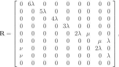
This is nothing more than aPH distribution with representation(~γ,G), where ~γ = [1,0,0,0,0,0,0,0], and
G=
−6λ 6λ 0 0 0 0 0 0
0 −5λ 5λ 0 0 0 0 0
0 0 −4λ 4λ 0 0 0 0
0 0 0 −3λ 3λ 0 0 0
0 0 0 0 −2λ−µ 2λ µ 0
0 0 0 0 0 −λ−µ 0 µ
ν 0 0 0 0 0 −2λ−ν 2λ
ν 0 0 0 0 0 0 −λ−ν
.
Example 2.9(AbsorbingCTMCs that do not representPH distributions). Not every
ab-sorbingCTMC can be used as a PHrepresentation. Consider the absorbingCTMCs depicted in Figure 2.3.
1 2
3 4
(a)
1 2 3
4 5 6 (b) 1 6 1 3 1 6 1 3
3 1 2
1
2.5. Phase-Type Distributions 15
The absorbingCTMC in Figure 2.3(a) is not a PH representation because it has more
than one absorbing state. The two states, of course, can always be collapsed or lumped together into one state, and thereby losing their identities; but this is not always desirable, for the identities might be important. The distribution of the time to absorption to state4
in thisCTMC, for instance, is not a probability distribution.
Figure 2.3(b), on the other hand, depicts an absorbing CTMC with a single absorbing
state. However, thisCTMCcontains 3 non-transient states, namely states3,4and5. These
are the states from which no path leading to the absorbing state exists. The probability of eventual absorption to state6, then, is not equal to 1. The CTMC is, therefore, not a PH
representation of any PH distribution.
Structural Definition The underlying absorbingCTMCof aPHrepresentation withn tran-sient states can be viewed as a tupleM = (S,R, ~π), where S = {s1, s2,· · · , sn, sn+1}
is the state space, Ris a rate matrix R : (S × S) → R≥0 of the underlying CTMC and
~π:S →[0,1]is the initial probability distribution on the state spaceS.
Now, apath σinMwith the absorbing statesais an alternating finite sequence of
states and their total outgoing rates
σ = s1
E(s1)
−−−−→s2
E(s2)
−−−−→s3
E(s3)
−−−−→ · · · E(sm−1)
−−−−−−→sm
E(sm)
−−−−→sm+1 =sa,
such that ~π(s1) > 0, sm+1 = sa, and satisfying R(si, si+1) > 0 for all 1 ≤ i ≤ m.
Let P aths(M) denote the set of all paths in M. With each path σ ∈ P aths(M), a probability
P(σ) =~π(s1)
m
Y
i=1
R(si, si+1)
E(si)
,
is associated. This probability is called the occurrence probability of the path. Intu-itively, the occurrence probability gives the probability of observing a particular path if the Markov process is run until it hits the absorbing state.
Example 2.10. The underlying CTMC of the PH representation(~γ,G) in Example 2.8 is
M= (S,R, ~π), whereS ={6,5,4,3,2,1, z1, z2, crash},
R=
0 6λ 0 0 0 0 0 0 0
0 0 5λ 0 0 0 0 0 0
0 0 0 4λ 0 0 0 0 0
0 0 0 0 3λ 0 0 0 0
0 0 0 0 0 2λ µ 0 0
0 0 0 0 0 0 0 µ λ
ν 0 0 0 0 0 0 2λ 0
ν 0 0 0 0 0 0 0 λ
0 0 0 0 0 0 0 0 0
,
and~π= [~γ,0]. One of the shortest pathsσs ∈P aths(M)in theCTMC is
16 Chapter 2. Preliminaries
The occurrence probability of pathσs is
P(σs) =~π(6)·
R(6,5)
E(6) ·
R(5,4)
E(5) ·
R(4,3)
E(4) ·
R(3,2)
E(3) ·
R(2,1)
E(2) ·
R(1, crash)
E(1) ,
= 1· 6λ
6λ ·
5λ
5λ ·
4λ
4λ ·
3λ
3λ ·
2λ
2λ+µ·
λ λ+µ =
2λ2
2λ2+ 3λµ+µ2 =
2
10302.
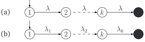
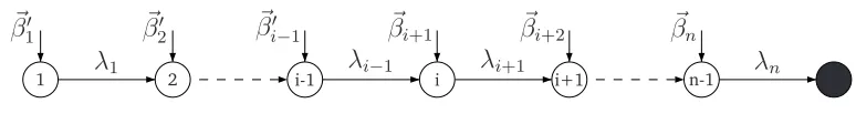
Let aPH-generator of the form
−λ1 λ1 0 · · · 0
0 −λ2 λ2 · · · 0
0 0 −λ3 · · · 0
..
. ... ... . .. ...
0 0 0 · · · −λn
be denoted byBi(λ1, λ2,· · ·, λn). APHrepresentation havingPH-generator of the form
Bi(λ1, λ2,· · · , λn)is called abidiagonal representation.
A path σ ∈ P aths(M) can be regarded as a PH distribution with representation
(~e1,Bi(E(s1), E(s2),· · ·, E(sm))), where vector ~e1 is a unit vector at the first
compo-nent of appropriate dimension. Let PH(σ) be the PH distribution of the path, namely
PH(σ) = PH(~e1,Bi(E(s1), E(s2),· · · , E(sm))). Now, we can put forward the following
proposition.
Proposition 2.11. Let the underlying absorbing continuous-time Markov chain of a
phase-type representation(~α,A)beM= (S,R, ~π). Then
PH(~α,A) = X
σ∈P aths(M)
P(σ)PH(σ).
Intuitively, a PH representation is characterized by the collection of its paths and
the probability with which each path occurs in the representation. It is straightforward thatPσ∈P aths(M)P(σ) = 1. Therefore, aPH representation is a convex combination of
its paths.
2.5.1
General Notions and Concepts
Cumulative and Density Functions Let~p(t)be the transient probability vector of the tran-sient states of a Markov chain representing PH distribution PH(~α,A), namely ~pi(t) is
the probability that the process is in state si, for1 ≤ i≤ n, at timet. Based on
Equa-tion (2.4), this transient probability vector satisfies the following system of differential equations
d
dt~p(t) =~p(t)A, t∈R+, (2.9)
with initial condition~p(0) =~α.
The solution of Equation (2.9) is~p(t) =~αeAt. Since the probability that the process
is in statesn+1(i.e., being in the absorbing state) at timetis the same as the probability
of not being in any of the states{s1, s2,· · · , sn}at timet, the distribution function of
the time until absorption in the Markov chain (hence ofPH distribution) is
2.5. Phase-Type Distributions 17
ThePH distribution is completely characterized by this (cumulative) distribution
func-tion.
From Equation (2.10), the probability density function of thePH distribution is
f(t) = d
dtF(t) =−αe~
AtA
~e=αe~ AtA,~ t∈R+. (2.11)
The PH distribution has a mass of αn+1 at t = 0. This means that the CTMC starts
immediately in the absorbing state with probabilityαn+1.
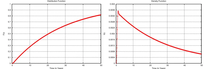
Example 2.12. Figure 2.4 depicts the curve of the distribution and respectively the density
functions ofPH(~γ,G)from Example 2.8.
0 0.1 0.2 0.3 0.4 0.5 0.6 0.7 0.8 0.9 1
0 10 20 30 40 50
F(t)
Time (in Years) Distribution Function
0 0.0004 0.0008 0.0012 0.0016 0.002 0.0024 0.0028 0.0032 0.0036 0.004
0 10 20 30 40 50
f(t)
Time (in Years) Density Function
Figure 2.4: PH Distribution (Left) and Density (Right) Functions
A PH distribution has no mass att = 0ifαn+1 = 0. A point mass at zero, namely a
probability distribution with a distribution functionF(t)such thatF(0) = 1, is a trivial
PH distribution, denoted byδ.
Irreducible Representations AllPHrepresentations we are dealing with in this thesis are
assumed to be irreducible. An irreducible representation is characterized as the repre-sentation in which no transient state is visited with probability zero for the specified initial probability distribution.
The irreducibility of a PH representation(~α,A) can be determined as follows. Let the underlying absorbing CTMC of (~α,A) be M = (S,R, ~π). For each state si ∈ S
such that ~π(si) > 0, we create a new transition with an arbitrary rate λ ∈ R+ from
the absorbing state to state si. Now, PH representation (~α,A) is irreducible if and
only if the newly modifiedCTMC is strongly connected. Recall that aCTMC is strongly connected if it is always possible to reach all states from any state.
If (~α,A) is an irreducible representation, each component of vector ~p(t) = ~αeAt
is strictly positive fort ∈ R+. On the other hand, if representation (~α,A) is not
irre-ducible, some components of~p(t)will be zero for allt ∈R≥0. In this case, all columns
of ~α and all rows and columns of A that correspond to the components of vector
~p(t) that are zero for all t ∈ R≥0 can be deleted to obtain the irreducible
18 Chapter 2. Preliminaries
Laplace-Stieltjes Transforms and Moments Aside from its distribution function, a PH
dis-tribution is also completely characterized by its Laplace-Stieltjes transform (LST). The
LST of the PH distribution is
˜
f(s) =
Z ∞
−∞
e−stdF(t) =α~(sI−A)−1A~+αn+1, s∈R≥0, (2.12)
whereIis then-dimensional identity matrix. This transform is a rational function,i.e.,
˜
f(s) =α~(sI−A)−1A~+αn+1 =
p(s)
q(s),
for some polynomialsp(s)andq(s)6= 0. When theLST is expressed in irreducible ratio,
the degree of the numeratorp(s)is no more than the degree of the denominatorq(s). The degrees of the two polynomials are equal only when vector~αis sub-stochastic but not stochastic [O’C90].
TheLST of an exponential distribution with rateλ∈R+ is given by
˜
f(s) = λ
s+λ. (2.13)
In the rest of the thesis, we sometimes refer to theLSTof aPHrepresentation. In this
case, we are actually referring to theLST of the PH distribution of the representation.
Example 2.13. The LST of PH distributionPH(~γ,G) described in Example 2.8 is given
byf˜(s) = pq((ss)), where
p(s) = 720(s+ 132)(s+ 83), and
q(s) = s8+ 236s7+ 17446s6+ 433436s5+ 5232949s4+ 34788584s3
+ 129998724s2+ 232835184s+ 7888320.
The rational functionf˜(s)shown above is expressed in irreducible ratio. The degree of its numerator is 2, while the degree of its denominator is 8.
Let PH(α,~ A) be the distribution of a random variable X. The k-th non-central moment ofPH(~α,A)is given by
mk =E[Xk] = (−1)kk!α~A−k~e, (2.14)
whereE[X]is the expected value of random variableX. The relationship between the
LST and the moments is described by
mk = (−1)k
dkf˜(s)
dsk
s=0
. (2.15)
2.5.2
Order and Degree
For aPH distribution with representation(~α,A), thesize of the representationis defined to be the dimension of matrixA. The degree of the denominator polynomial of itsLST
2.5. Phase-Type Distributions 19
are called the poles of the LST. Sometimes we also call them the poles of the PH
distribution.
It is known [Neu81, O’C90] that a given PH distribution has more than one
rep-resentation. The size of aminimal representation—namely a representation with the least number of states—is called the order of the phase-type distribution. Note that in standard literature, the size of a representation is called the order of the representa-tion. We choose to call it “size” to avoid confusion with the order of aPH distribution.
The order of a PH distribution may be different from its algebraic degree but it is no less than its algebraic degree [O’C90]. The following lemma is straightforward.
Lemma 2.14. A phase-type representation whose size is equal to the algebraic degree of
its phase-type distribution is a minimal representation.
In this case, the order of the distribution is then simply given by the size of the representation.
Example 2.15. We continue using the PH distribution described in Example 2.8, whose
representation is (~γ,G). The size of the representation is the dimension of G, i.e., 8. Now, the algebraic degree of thePHdistribution is given by the degree of the denominator polynomial of its LST, which in this case is also 8. The poles of the LST are given by
the zeros of q(s), and they are s = −3.329344±4.307561ı, s = −8.753829±2.893837ı,
s=−0.034539,s=−8.799086,s=−101.00005ands=−101.999975.
Since the size of the representation is equal to the algebraic degree of the distribution,
(~γ,G)is a minimal representation. Therefore, the order of the distribution PH(~γ,G) is also 8.
In this thesis, PH distributions whose order is equal to their algebraic degree play
an important role. The following definition simplifies the way we refer to them.
Definition 2.16. A phase-type distribution is calledidealif and only if its order is equal
to its algebraic degree.
2.5.3
Dual Representations
Let{Xt |t∈R≥0}be an absorbing Markov process representing aPH distribution and
letτ be a random variable denoting its absorption time.
Definition 2.17([Kel79]). Thedualor thetime-reversalrepresentation of the absorbing
Markov process{Xt |t∈R≥0}is given by an absorbing Markov process{Xτ−t |t∈R≥0}.
The relationship between the two processes can be described intuitively as follows: the probability of being in state s at time t in one Markov process is equal to the probability of being in state s at time τ −t in the time-reversal Markov process and vice versa.
Theorem 2.18 ([CC93, CM02]). Given a PH representation (~α,A), then its dual
repre-sentation is(β,~ B)such that ~
β =A~⊤M and B=M−1A⊤M, (2.16)
20 Chapter 2. Preliminaries
Recall that A~ in Equation (2.16) is a column vector representing the rates of the transitions from all transient states to the absorbing state. From Equation (2.16), we can derive that
~
B =M−1~α⊤. (2.17)
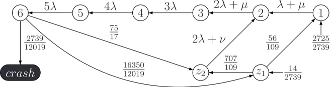
Example 2.19. Figure 2.5 depicts the dual or time-reversal of the representation shown
in Figure 2.2. Several transition rates and initial probabilities are written as rational numbers rather than as expressions ofλ,µ, and/orν, because they are simply too long to be printed. Recall from Example 2.8 thatλ = 1, µ= 100, andν = 6. For the remaining transitions, the rates are expressed inλ,µ, and/orν so that the correspondence between the original and the dual representations can be observed.
crash
6 5 4 3 2 1
2725 2739
z2 z1 273914 2739
12019
5λ 4λ 3λ 2λ+µ λ+µ
2λ+ν 56
109 707
109 75
17
16350 12019
Figure 2.5: The Dual of the Representation in Figure 2.2
From the form of Equation (2.16) as well as from the example, several properties of the dual representation can be inferred: (1) the dual representation has the same number of states as the original one; (2) there is a one-to-one correspondence between the state spaces of the two representations: a state in Figure 2.2, for instance, corre-sponds to a state with the same identity in Figure 2.5, and these states have the same total outgoing rate; (3) the dual representation is the reverse of the original represen-tation,i.e., the direction of each transition that does not end in the absorbing state is reversed in the dual, each state with a transition to the absorbing state in the original becomes a state with nonzero initial probability in the dual, and conversely each state with nonzero initial probability in the original becomes a state with a direct transition to the absorbing state in the dual; and (4) both representations represent the samePH
distribution.
2.5.4
Characterization
All PH distributions have rational Laplace-Stieltjes transforms. However, not every
probability distribution with rationalLST is aPHdistribution. For instance, some mem-bers of matrix-exponential distributions [AB96, AO98, Fac03, HZ07b]—which we will discuss further in Section 2.8—are notPHdistribution. The following characterization
theorem establishes the necessary and sufficient conditions for a probability distribu-tion to be aPH distribution.
Theorem 2.20 ([O’C90]). A probability distribution defined on R≥0 is a phase-type
dis-tribution if and only if it is the point mass at zero (δ), or it satisfies the following condi-tions:
2.5. Phase-Type Distributions 21
2. its Laplace-Stieltjes transform is a rational function having a real pole whose real part is strictly larger than the real parts of all other poles.
Therefore, any probability distribution whose density function is equal to zero at somet ∈R+is not aPH distribution. Moreover, aPH distribution must have a rational
LST with a real pole whose real part is strictly larger than the real parts of all other poles. This means that the largest real pole is unique. An LST with a complex pole whose real part is the largest is not theLSTof aPHdistribution, since there are then two
poles having the largest real part, for its conjugate is also a pole. From Example 2.15, for instance, we know that the probability distribution associated with representation
(~γ,G) has an LST with a unique real pole having the largest real part, namely s =
−0.034539. Hence, it is a PH distribution.
Example 2.21 (Not a phase-type). A probability distribution with density function
f(t) =e−t+e−tcos(t)is not aPH distribution. The LST of the distribution is
˜
f(s) = 2s
2+ 4s+ 3
(s+ 1)(s2+ 2s+ 2),
and the poles ares=−1,s =−1 +ı, ands=−1−ı. Hence, the LST has no unique real
pole whose real part is the largest among the real parts of all poles.
Any probability distribution that fails to satisfy any of the two conditions is not a PH distribution. It is interesting to note, however, that as a PH distribution more
nearly fails to satisfy the second condition—namely its LST has poles whose real part approaches the largest one—more states are required to represent it [O’C91].
2.5.5
Closure Properties
The set of allPHdistributions isclosedunder a certain operation if the application of the operation on anyPH distributions produces a PH distribution. The set of all such
oper-ations defines the closure properties ofPH distributions. Some of these closure
proper-ties can be found in [Neu81]. Closure properproper-ties under four operations—convolution, minimum, maximum, and mixture—are required in this thesis.
Definition 2.22. Let p ∈ R≥0 and 0 ≤ p ≤ 1. For two distribution functions F(t) and
G(t), let the distribution functions:
(a) con(F(t), G(t)) = [F ∗G](t) =R0tF(t−x)G(x)dx,
(b) min(F(t), G(t)) = 1−(1−F(t))(1−G(t)),
(c) max(F(t), G(t)) =F(t)G(t), and
(d) mix(pF(t),(1−p)G(t)) =pF(t) + (1−p)G(t).
We refer to these functions as the convolution, minimum, maximum, and mixture,2 respectively, of the two distributions.
2Note that there is an inconsistency in our naming: convolution and mixture operations proceed
22 Chapter 2. Preliminaries
The following theorem establishes that the set of PH distributions is closed under
the four operations. The theorem also provides the representation of the PH distribu-tion produced by each of the operadistribu-tions.
Theorem 2.23([Neu81]). LetF(t)andG(t)be two phase-type distributions with
repre-sentations(~α,A)and(β,~ B)of sizemandn, respectively. Then:
(a) con(F(t), G(t))is a phase-type distribution with representation(~δ,D)of sizem+n, where
~δ= [~α, αm+1β~] and D=
A A~~β ~0 B
. (2.18)
(b) min(F(t), G(t))is a phase-type distribution whose representation is3
(α~⊗β,~ A⊕B), (2.19)
of sizemn.
(c) max(F(t), G(t))is a phase-type distribution with representation(~δ,D)of sizemn+
m+n, where
~δ=h α~ ⊗β, β~ n+1~α, αm+1β~
i
and
D=
A⊕B Im⊗B~ A~⊗In
0 A 0
0 0 B
. (2.20)
(d) mix(pF(t),(1−p)G(t)) is a phase-type distribution with representation (~δ,D) of sizem+n, where
~δ= [p~α,(1−p)β~] and D=
A 0
0 B
. (2.21)
In the following definition, we abuse the notation of convolution, minimum, maxi-mum, and mixture functions to not only operate onPH distributions, but also to
oper-ate on the representations ofPH distributions.
Definition 2.24. For two phase-type representations(α,~ A)and(β,~ B), let the functions:
(a) con((α,~ A),(β,~ B)) = (~δ,D)as given in Equation(2.18),
(b) min((~α,A),(β,~ B)) = (~α⊗β,~ A⊕B)as given in Equation(2.19),
(c) max((~α,A),(β,~ B)) = (~δ,D)as given in Equation(2.20), and
(d) mix(p(~α,A),(1−p)(β,~ B)) = (~δ,D)as given in Equation(2.21).
We refer to these functions as the convolution, minimum, maximum, and mixture, re-spectively, of the two phase-type representations.
3See Appendix A.2 for the definitions of the Kronecker product (
2.6. Acyclic Phase-Type Distributions 23
The convolution, minimum, and maximum operations on PH distributions (and
also onPH representations) are commutative and associative.
Let F(t) be a probability distribution on R≥0, and let X be a random variable
governed by a geometric distribution with parameterp ∈ R≥0, 0 ≤ p < 1. We define
F(t)(p)as the distribution of the sum ofX+ 1independent and identically distributed
random variables with distributionF(t), namely
F(t)(p) := (1−p) F(t) +pF(t)∗F(t) +p2F(t)∗F(t)∗F(t) +· · ·,
where∗denotes the convolution of two probability distributions.
Intuitively, operationF(t)(p) is a kind of tail-recursion on probability distributions.
If F(t) is a PH distribution, the operation produces another PH distribution whose
underlying Markov process repeatedly performs a trial when it is about to hit the absorbing state in order to decide whether to restart the process with probability1−p, or to hit the absorbing state with probabilityp. The set ofPHdistributions is also closed
under this operation.
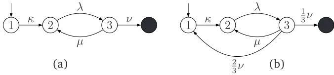
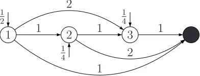
Figure 2.6 illustrates the effects of the operation on the representation of a PH
distribution. Figure 2.6(a) depicts a PH representation of F(t), and Figure 2.6(b)
depicts aPH representation ofF(t)(13).
1 κ 2 3
λ
µ
ν
(a)
1 κ 2 3
λ
µ
1 3ν
2
3ν (b)
Figure 2.6: OperationF(t)(p)on Phase-Type Representation
Some of the closure properties are enough to characterize the set of allPH
distribu-tions [MO92], as described in the following theorem.
Theorem 2.25 ([MO92]). The family of phase-type distributions is the smallest family
of distributions on R≥0 that:
1. contains the point mass at zero (δ) and all exponential distributions,
2. is closed under finite mixture and convolution,
3. is closed under the operationF(t)(p), for0≤p <1.
The theorem establishes that the whole family ofPH distributions can be generated by the point mass at zero and exponential distributions together with the finite mixture, convolution, and recursion (restart