Wiley Digital Signal Processing Techniques And Applications In Radar Image Processing Aug 2008 ISBN 0470180927 pdf

(1)

(2)

DIGITAL SIGNAL

PROCESSING

TECHNIQUES AND

APPLICATIONS IN RADAR

IMAGE PROCESSING

Bu-Chin Wang

(3)

(4)

WILEY SERIES ON INFORMATION AND COMMUNICATIONS TECHNOLOGIES Series Editors: Russell Hsing and Vincent K. N. Lau

The Information and Communications Technologies (ICT) book series focuses on creating useful connections between advanced communication theories, practical designs, and end-user applications in various next generation networks and broadband access systems, includ-ing fiber, cable, satellite, and wireless. The ICT book series examines the difficulties of applying various advanced communication technologies to practical systems such as WiFi, WiMax, B3G, etc., and considers how technologies are designed in conjunction with stan-dards, theories, and applications.

The ICT book series also addresses application-oriented topics such as service manage-ment and creation and end-user devices, as well as the coupling between end devices and infrastructure.

T. Russell Hsing, PhD, is the Executive Director of Emerging Technologies and Services Research at Telcordia Technologies. He manages and leads the applied research and devel-opment of information and wireless sensor networking solutions for numerous applications and systems. Email: thsing@telcordia.com

Vincent K.N. Lau, PhD,is Associate Professor in the Department of Electrical Engineering at the Hong Kong University of Science and Technology. His current research interest is on delay-sensitive cross-layer optimization with imperfect system state information. Email: eeknlau@ee.ust.hk

Wireless Internet and Mobile Computing: Interoperability and Performance Yu-Kwong Ricky Kwok and Vincent K. N. Lau

RF Circuit Design Richard C. Li

(5)

DIGITAL SIGNAL

PROCESSING

TECHNIQUES AND

APPLICATIONS IN RADAR

IMAGE PROCESSING

Bu-Chin Wang

(6)

No part of this publication may be reproduced, stored in a retrieval system, or transmitted in any form or by any means, electronic, mechanical, photocopying, recording, scanning, or otherwise, except as permitted under Section 107 or 108 of the 1976 United States Copyright Act, without either the prior written permission of the Publisher, or authorization through payment of the appropriate per-copy fee to the Copyright Clearance Center, Inc., 222 Rosewood Drive, Danvers, MA 01923, (978) 750-8400, fax (978) 750-4470, or on the web at www.copyright.com. Requests to the Publisher for permission should be addressed to the Permissions Department, John Wiley & Sons, Inc., 111 River Street, Hoboken, NJ 07030, (201) 748-6011, fax (201) 748-6008, or online at http://www.wiley.com/go/permissions. Limit of Liability/Disclaimer of Warranty: While the publisher and author have used their best efforts in preparing this book, they make no representations or warranties with respect to the accuracy or completeness of the contents of this book and specifically disclaim any implied warranties of merchantability or fitness for a particular purpose. No warranty may be created or extended by sales representatives or written sales materials. The advice and strategies contained herein may not be suitable for your situation. You should consult with a professional where appropriate. Neither the publisher nor author shall be liable for any loss of profit or any other commercial damages, including but not limited to special, incidental, consequential, or other damages.

For general information on our other products and services or for technical support, please contact our Customer Care Department within the United States at (800) 762-2974, outside the United States at (317) 572-3993 or fax (317) 572-4002.

Wiley also publishes its books in a variety of electronic formats. Some content that appears in print may not be available in electronic formats. For more information about Wiley products, visit our web site at www.wiley.com.

Library of Congress Cataloging-in-Publication Data

Wang, Bu-Chin.

Digital signal processing techniques and applications in radar image processing / Bu-Chin Wang. p. cm.

ISBN 978-0-470-18092-1

1. Signal processing—Digital techniques. 2. Remote sensing. I. Title. TK5102.9.W36 2008

621.36′_78–dc22

2008004941 Printed in the United States of America

(7)

To my mother Chun-Ying Wang, in memory of my father Lan-Din Wang, and

(8)

(9)

PREFACE

In the past few decades, the principles and techniques of digital signal processing (DSP) have been used in applications such as data and wireless communication, voice and speech analysis and synthesis, and video and image compression and ex-pansion. Radar image processing is considered the primary application of the remote sensing field and is a new and emerging area for DSP applications. Although the primary application of satellite-based radar imaging is military surveillance, the low cost and real-time processing capability of radar imaging, together with its capability to operate under any environmental conditions (e.g., night or day, rain or snow, fog or clear sky) have opened up many commercial applications. Sea ice monitoring and disaster monitoring of events such as forest fires, floods, volcano eruptions, earth-quakes, and oil spills are examples of satellite-based radar imaging applications. Airborne-based radar systems also have made radar imaging more affordable and popular. Furthermore, exploration of underground natural resources is an example of a new application.

The processing of radar images, in general, consists of three major ﬁelds: DSP principles and communication theory, knowledge of antenna and radar operation, and algorithms used to process the radar images. The purpose of this book is to include the material in these ﬁelds in one publication, to provide the reader with a thorough understanding of how radar images are processed. To further familiarize the reader with the theories and techniques used in processing radar images, MATLAB*_-based

programs are utilized extensively in this book in both the synthesis and analysis of the radar image. In this way, the signal waveforms are therefore made visible at various stages during computer simulation, and the capability of three-dimensional (3D) graphical displays makes many abstract results easier to understand. This book is aimed at engineers or students who have some knowledge of DSP theory and limited knowledge of communication theory and/or antenna theory, but are interested in advanced DSP applications, especially in the remote sensing ﬁeld.

This book consists of three major groups of chapters. Chapters 1 and 2 pro-vide an overview of DSP principles, reviewing signal characteristics in both analog and digital domains and describing some DSP techniques that serve as key tools in radar images processing. Chapters 3–5 discuss the basics of antenna theory, radar

*_{MATLAB is a registered trademark of math Works, Inc., Natick, MA 01760.}

(16)

xiv PREFACE

operation principles, modulation/demodulation, and radar target detection tech-niques. Chapters 6–9 discuss the properties and formation of radar images and then try to model the processing of radar images. The principles of radar image data syn-thesis are presented and demonstrated with computer-simulated examples. Both the range–Doppler and the Stolt interpolation algorithms are described and applied to the simulated image data and satellite radar-based image data. The results are analyzed and compared. MATLAB∗ _{programs are used extensively during the generation of}

various waveforms of signal processing, radar detection, and synthesis/simulation of radar image processing.

The first two chapters briefly review the DSP principles. Chapter 1 describes the characteristics of signals, followed by Fourier series representation of periodic sig-nals. Fourier transform is then introduced to represent a signal, whether in periodic or nonperiodic form. Sampling theory and interpolation filter are derived, and some advanced sampling and interpolation techniques are reviewed. Resampling from un-evenly spaced data to obtain un-evenly spaced data is briefly discussed at the end of the chapter. Chapter 2 addresses the discrete signal transformation in both time and fre-quency domains. Discrete Fourier transform (DFT), together with some of its charac-teristics, are reviewed. Windowing functions and the well-known fast Fourier trans-form (FFT) technique are covered. The discrete cosine transtrans-form (DCT), which is the byproduct of DFT, is introduced. A graphical representation of DFT provides an overview of the relationship between a continuous signal and a discrete signal. It also provides signal variations in both time and frequency domains. The chapter ends with an example of resampling with fractional interpolation based on DFT technique.

Chapters 3–5 provide a background review on antenna theory and radar operation principles. Chapter 3 starts the review of the electromagnetic field with the Maxwell equation, followed by the electromagnetic (EM) fields generated from the infinitesi-mal dipole. Finite-length dipole- and half-wavelength dipole-based linear antenna ar-rays are described. Some commonly used antennas, including the microstrip antenna, are also covered. Chapter 4 deals with the basic theory of radar signal processing. The radar range equations and other related parameters are reviewed. The Doppler fre-quency due to relative movement between radar and target is briefly discussed with respect to the wavefront. Some target range and motion direction detection tech-niques are also revealed at the end of chapter. Chapter 5 provides broad coverage of modulation/demodulation and target detection techniques used by radar systems. Amplitude modulation (AM)-based pulse Doppler frequency radar is first reviewed, followed by discussion of target detection techniques. Frequency modulation (FM)-based radars, which include pulsed linear FM (LFM), continuous-wave LFM and stepped LFM signals, are then briefly discussed. Also covered in this chapter are in-phase–quadrature-phase (I–Q) demodulator and pulse compression (or matched filtering), which serve as important tools in radar signal processing

(17)

PREFACE xv

migraion, geometric distortion, and resolution of image radar. Chapter 7 discusses the ideal system model of radar imaging. The reconstruction of 2D target function is modeled by two independent 1D functions. The model of 1D range imaging is ﬁrst described, followed by discussion of the 1D cross-range imaging. Data acquisition and the frequency spectrum of radar image are also reviewed. Chapter 8 discusses the principles of radar image generation and how to synthesize the radar image. Ex-amples of synthesizing radar image data for broadside SAR and squint SAR are presented, which include single and multiple targets. The range–Doppler algorithm on processing radar images is then reviewed and applied to the synthesized data. Chapter 9 reviews some radar image processing techniques in the wavenumber do-main. The Stolt interpolation technique on radar image processing is brieﬂy reviewed and applied to some simulated image data. The real satellite radar signal is then pro-cessed by both range–Doppler and Stolt interpolation algorithms. A comparison on these two algorithms is also provided.

Some of the material in this book was presented to graduate students in Su-Zhou University in China, and the feedback from the students was incorporated into this book. It is my hope that this book can provide enough knowledge for readers to become familiar with radar image processing. Although I have made every effort to make this a thorough and accurate book, errors and mistakes are inevitable. Any comments or feedback from readers will be welcomed and appreciated.

Acknowledgment

I would like to thank Dr. Russell Hsing of Telcordia for his support and inspiration throughout the process of writing this book. His advice made the publication of this book possible and is greatly appreciated.

Finally, I owe a lot to my family for their patience and understanding as I worked on this book. My wife, Rhoda, my children, Anna and David, my son-in-law, Scott Chong, and granddaughter, Jocelyn, all helped make this book possible in numerous ways, and I am grateful to them.

(18)

(19)

LIST OF SYMBOLS

As Azimuth sample spacing along the azimuth oryaxis, meters

␣ Frequency change rate for LFM signal, hertz per second (Hz/s) ␤ Frequency change rate for LFM signal along azimuth direction,

Hz/s

B,Bt Frequency bandwidth, Hz BD,BDop Doppler frequency bandwidth, Hz

BDs Doppler frequency bandwidth in terms of slow times, Hz BDu Doppler frequency bandwidth in terms of radar positionu, Hz Bku Spatial frequency bandwidth in thekudomain, Hz

c Speed of light, 3×108_{meters per second (m/s)} f Frequency, Hz

fb Baseband frequency, Hz f0 Reference frequency, Hz fc Carrier frequency, Hz fs Sampling frequency, Hz fm Maximum frequency, Hz fPRF Pulse repetition frequency, Hz fD Doppler frequency, Hz

fDr Doppler frequency in terms of slant ranger, Hz fDs Doppler frequency in terms of slow times, Hz fDu Doppler frequency in terms of radar positionu, Hz fDc Centroid of Doppler frequency, Hz

fDcr fDcwith respect to slant ranger, Hz fDcs fDcwith respect to slow times, Hz fDcu fDcwith respect to radar positionu, Hz

˙

fDcs Derivative of fDcs, or slope of fDcs, Hz/s

˙

fDc Derivative of fDc, or slope of fDc, Hz/s

˙

fD Derivative of fD, or slope of fD, Hz/s

fDU Upper bound of Doppler frequency bandwidth, Hz fDL Lower bound of Doppler frequency bandwidth, Hz fDUr fDUwith respect to slant ranger, Hz

fDLr fDLwith respect to slant ranger, Hz fDUs fDUwith respect to slow times, Hz

(20)

xviii LIST OF SYMBOLS

fDLs fDLwith respect to slow times, Hz f0(x) Ideal target function along range orxaxis f0(y) Ideal target function along azimuth oryaxis f(x) Target function along range orxaxis

f(y) Target function along azimuth oryaxis

F0(k) Fourier transform of f0(x) F0(ky),F0(ku) Spatial Fourier transform of f0(y) F(k) Fourrier transform of f(x)

F(ky),F(ku) Spatial Fourier transform of f(y) hr(t) Range matched ﬁlter

haz(s) Azimuth matched ﬁlter haz(t,s) 2D azimuth matched ﬁlter

Haz(␻,␻D) 2D spatiotemporal Fourier transform ofhaz(t,s)

Im(ku) Gating function in wavenumberkudomain due tomth target im(u) Inverse spatial Fourier transform ofIm(ku)

kx Spatial wavenumber, corresponding to spatial Fourier transform of x, 1/meter (m−1; reciprocal meter)

ku Spatial wavenumber, corresponding to spatial Fourier transform of u, m−1

kum Spatial wavenumber, corresponding tomth target k′

u Spatial wavenumber changing rate ky Same asku, m−1

k Wavenumber, corresponding to f, m−1

kb Wavenumber in baseband corresponding to fb, m−1 k0 Wavenumber, corresponding to f0, m−1

kc Wavenumber, corresponding to fc, m−1

␭ Wavelength of electromagnetic wave, m

L Antenna length, m

Ls Synthetic aperture length, m

Lsa Lsfor target located at range R0a, m Lsa2 Half size ofLsa, m

Lsx Lsfor target located at range R0xforx=b,c,d . . . ,m Lsx2 Half size ofLsx, m

Lsai Lsaforith target

Lsxi Lsxforith target

Ltotal Sum ofLsxfrom all targets, m M Number of rows in a 2D data array

Mamb Doppler ambiguity

N Number of columns in a 2D data array

Naz Number of azimuth lines within the synthetic aperture lengthLs Nazi Number of azimuth lines withinLsfor target located at rangeR0i Nr Number of samples within the transmitter pulse duration

Nr x Number of sample difference between rangeRx, forx=b,c. . .,

(21)

LIST OF SYMBOLS xix

P(␻) Fourier transform ofp(t)

pb(t) Baseband transmitted radar signal

psf(t) Pont spread function in time domain psf(␻) Fourier transform of psf(t)

R0 Shortest distance between target and radar, m R0a R0with target located at rangex=a, m R0i R0with target located at rangex=b,c. . ., m Ruin Slant range between targetnand radar located atui, m

Rc Distance between target and radar when target is under

illunination of radar center beam, m

R1 Distance between target and radar when radar starts to illuminate

the target, m

R3 Distance between target and radar when radar stops to illuminate

the target, m

Rs Slant range sample spacing, m

RS shortest distance from radar to ground along the range (x-axis)

direction, m

RL Longest distance from radar to ground along the range (x-axis)

direction, m

R(s) Slant range in terms of slow times, m

R(u) Slant range in terms of radar positionu, m

⌬R Slant range difference with respect toR0(broadside SAR case) or R3(squint SAR case), m

⌬Rr Slant range resolution, m

⌬Rgr Ground range resolution, m

⌬Ra Angular resolution, m

s Slow time variable along radar moving direction, seconds (s)

sc Slow time when target is illuminated by center beam of radar, s s(t) Target reﬂected signal

sb(t) Baseband signal ofs(t) S(␻) Fourier transform ofs(t)

Sb(␻) Fourier transform ofsb(t)

S(t,u) Target reﬂected signal when radar is at locationy=u S(␻,␻D) 2D Spatiotemporal Fourier transform ofs(t,u)

sm(t,u) mth target reﬂected signal when radar is at locationy=u Sm(␻,␻D) 2D spatiotemporal transform ofsm(t,u)

sbm(t,u) Baseband version ofsm(t,u) Sbm(␻,␻D) Baseband version ofSm(␻,␻D)

sr0(u) Range reference fouction for radar located at (0,u) Sr0(ku) Spatial Fourier transform ofsr0(u)

␶ Pulse duration time or echo delay time, s ␶ui Echo delay time when radar is located atui, s

␶uin Echo delay time due to targetnand when radar is located atui, s

T,T0 Period of periodic signal, s

(22)

xx LIST OF SYMBOLS

Tp Pulse duration time, s

u Radar position variable along the azimuth oryaxis, m

ui Radar position atu =ui, m

u2 Radar location when target is under illumination of radar center

beam, m

u1 Radar location when radar begins to illuminate target, m u3 Radar location when radar ceases to illuminate target, m V Radar velocity, a vector along azimuth direction m/s

Vr Radar’s radial velocity, a scalar along the target direction, m/s W Antenna width, m

Xc Centerpoint of target area alongxaxis, m

X0 Half size of target area along range (x-axis) direction, m Y0 Half size of target area along azimuth (y-axis) direction, m Yc Centerpoint of target area alongyaxis, m

yi Target location alongyaxis, m

⬍r n⬎ 2D signal array corresponding to targetn ␻ Angular frequency, Hz

␻b Angular baseband frequency, Hz

␻0 Angular reference frequency, Hz

␻c Angular carrier frequency, Hz

␴i Reﬂection coefﬁcient fromith target

␪ Angle, radians, or degrees

␪H Horizontal beamwidth=␭/L, radians or degrees

␪V Vertical beamwidth=␭/W, radians or degrees

␪3dB Antenna 3-dB beamwidth, radians or degrees

␪m(u) Aspect angle with respect tomth target when radar is at location y=u, radians or degrees

␪u Equal to␪m(u) for single target

␪q Radar squint angle, radians or degrees

␦(t) Delta or impulse function

sinc(t) Sampling or interpolation ﬁlter function

Rect(t) Time-domain rectangular pulse with duration|t_{| ≤} 1 2

|␹(␶, fD)| Radar ambiguity function

F _{Fourier transform operator} F−1 _{Inverse Fourier transform operator}

(23)

LIST OF ILLUSTRATIONS

Figures

1.1 A sinc (t) function. 2

1.2 A linear system. 3

1.3 Graphical representations of a function in terms of pulses. 3 1.4 A time-invariant linear system. 4 1.5 A periodic signalgp(t). 7

1.6 Fourier series coefﬁcients of a periodic pulse. 9 1.7 A single pulseg(t) and its Fourier transformG(␻). 14 1.8 A single-pulse frequency spectrumG(␻) and its inverse Fourier

transformg(t). 15

1.9 A periodic impulse train and its Fourier transform. 17 1.10 Fourier transform of a periodic pulse train. 19 1.11 Graphical representations of the sampling theory. 20 1.12 Interpolation ﬁlters. 22 1.13 Original and half-sample-shifted digital signals. 23 1.14 Frequency spectra of a digitized bandpass signal. 25 1.15 Downsampling with a FIR ﬁlter. 26 1.16 Interpolation with zero insertion and FIR LPF. 27 1.17 Fractional rate interpolation withM=2.5. 28 1.18 Interpolation on evenly spaced data. 30 1.19 Generation of unevenly spaced data index. 31 1.20 Relationship between evenly and unevenly spaced data. 32 1.21 Interpolation on unevenly spaced data. 33

2.1 A periodic sequence. 36

2.2 Linear convolution. 40

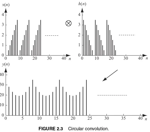
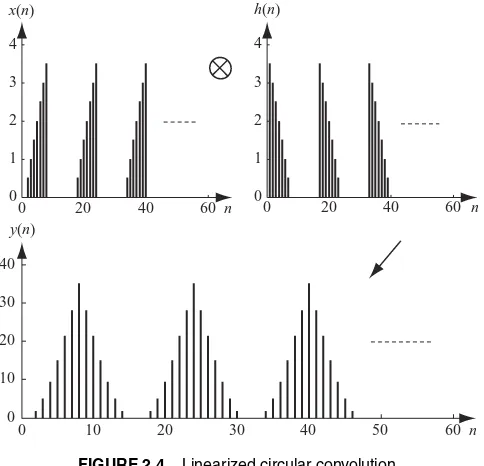
2.3 Circular convolution. 41 2.4 Linearized circular convolution. 42 2.5 Convolution using overlap-and-add method. 43

(24)

xxii LIST OF ILLUSTRATIONS

2.6 Convolution using overlap-and-save method. 44 2.7 Hanning window with different sampling frequencies. 45 2.8 A 32-point Hanning window. 46 2.9 Hanning window with time-domain zero padding. 46 2.10 Hanning window with frequency-domain zero padding. 47 2.11 DFT with sliding (overlapping). 49 2.12 Hamming and Blackman window functions. 50 2.13 Three-stage computation of an 8-point DFT. 52 2.14 An 8-point FFT with decimation-in-time algorithm. 52 2.15 First stage of the decimation-in-frequency FFT algorithm. 54 2.16 The 8-piont decimation-in-frequency FFT algorithm. 54 2.17 Input block (a) and end effects in DFT (b) and DCT (c). 56 2.18 Graphical representations of DFT. 59 2.19 Example of resampling. 61 3.1 Potentials generated by current/charge distribution. 66 3.2 Radiation from a point radiator. 67 3.3 Far-ﬁeld approximation ofz-oriented dipole. 71 3.4 Radiation pattern of a half-wavelength dipole. 74 3.5 A 10-element linear array. 75 3.6 Normalized linear antenna array factor forN=10. 77 3.7 Normalized linear antenna array factor forN=10,d=␭/2. 78 3.8 Field pattern in rectangular format forN=6. 81 3.9 Field pattern in polar format forN=6. 82 3.10 Graphical representation of a solid angle. 83 3.11 Antenna radiation pattern approximated as a rectangular area. 86 3.12 Antenna radiation pattern approximated as an elliptical area. 88

3.13 Polarized ﬁelds. 89

3.14 Popular antennas: (a) circular loop antenna; (b) linear polarized horn

antenna; (c) parabolic antenna. 90 3.15 Printed patch antenna. 91 3.16 Conﬁguration of a 4-dipole linear array. 92 3.17 Half-wavelength dipole-based 2D antenna array. 92 4.1 Transmitter and receiver pulse trains. 94 4.2 Pulse repetition period and range ambiguity. 95

4.3 Range resolution. 95

(25)

LIST OF ILLUSTRATIONS xxiii

4.7 Wave propagation for stationary source and stationary receiver. 103 4.8 Wave propagation for moving source and stationary receiver. 104 4.9 Wave propagation for stationary source and moving receiver. 105 4.10 Wave propagation for moving source and moving receiver. 106 4.11 Doppler radar with separate source and receiver. 107 4.12 Example of Doppler frequency. 109 4.13 Rectangular pulse and its frequency spectrum. 112 4.14 Ambiguity function of a rectangular pulse in 3D view. 113 4.15 Cross-sectional view of Fig. 4.14 with␶=0 (a) and␶=0.5Tp(b). 114

4.16 Cross-sectional view of Fig. 4.14 with fD=0 (a) and fD=2.5/Tp(b). 114

4.17 A 3-dB contour of ambiguity function of a rectangular pulse in 3D view. 115 5.1 Transmitter block diagram of a pulse-modulated radar system. 118 5.2 Time- and frequency-domain waveforms of pulse-modulated

radar signal. 119

5.3 Time- and frequency-domain waveforms of two video pulses. 120 5.4 Block diagram of Doppler frequency extraction. 121 5.5 Block diagram of an offset carrier demodulation. 122 5.6 Block diagram of a pulse–Doppler radar system. 122 5.7 Time-domain waveform (a) and time–frequency relation (b) of a

pulsed LFM signal. 125

5.8 Time- and frequency-domain waveforms of a pulsed symmetric

LFM signal. 128

5.9 Time- and frequency-domain waveforms of a pulsed nonsymmetric

LFM signal. 128

5.10 Block diagram of a PLFM radar system. 129 5.11 Block diagram of a CWLFM radar system. 129 5.12 Time–Frequency relationship of a CWLFM radar signal. 130 5.13 Waveforms of (a) a CWSFM radar signal and (b) a pulsed SFM

radar signal. 131

5.14 Time–frequency relationship of (a) CWSFM radar signal and (b) a

PSFM radar signal. 132

(26)

xxiv LIST OF ILLUSTRATIONS

5.23 Comparison of pulse compression based on convolution and DFT. 142 5.24 Waveforms of Tx signal and MF function. 143 5.25 Frequency spectra of Tx signal and MF function. 144 5.26 Time- and frequency-domain waveforms of Rx signal. 145 5.27 Comparison of pulse compression based on convolution and DFT. 146 5.28 Time–frequency relationship of Tx, reference, and echo signals. 147 5.29 Block diagram of dechirp processing. 147 5.30 Time–frequency relationship of Tx and echo signals from two

stationary targets. 148

5.31 Time–frequency relationship of Tx and echo signals from two moving

targets. 149

5.32 Baseband echo response from PSFM signal. 150 5.33 A single-target range profile based on PSFM signal. 151 5.34 Stepped frequency pulse train and echoes returned in one pulse period. 152 5.35 A multiple-target range profile based on PSFM. 153 6.1 Configurations of (a) a stripmap SAR and (b) a scan SAR. 156 6.2 Imaging radar for (a) a spotlight SAR and (b) an interferometric SAR. 156 6.3 Geometry of stripmap imaging radar. 157 6.4 Geometry of (a) a broadside SAR and (b) a squint SAR. 158 6.5 (a) Imaging radar and (b) radar pulse and received echo. 159 6.6 (a) Single channel radar range data; (b)M×Nradar imaging

data array. 161

6.7 Conﬁguration of a broadside SAR system. 162 6.8 A simpliﬁed broadside SAR system. 162 6.9 Echo signal from the point target before (a) and after (b)

range compression. 163

6.10 Broadside SAR with multiple targets. 164 6.11 Slant rangeR(u) versus radar positionufor three targets at equal (a)

and different (b) ranges. 164 6.12 Broadside SAR with single point target. 165 6.13 (a) Radiation pattern from a typical antenna array; (b) real part of a

LFM signal. 169

(27)

LIST OF ILLUSTRATIONS xxv

6.20 Low␪qDoppler frequency versus slow times(a) and slant ranger(b). 183

6.21 Comparison of Doppler frequencies for different SAR systems. 184 6.22 (a) Multiple-target squint SAR system; (b) plot of Doppler frequency

fDversus radar displacementu. 185

6.23 A simplified single-target squint SAR system. 186 6.24 Single-target trajectory in squint SAR system. 187 6.25 Geometric distortions of radar image. 188 6.26 The resolution cell of a side-looking radar. 190 7.1 Geometry of a range imaging radar. 195 7.2 An ideal target function. 195 7.3 Matched filtering for range imaging. 197 7.4 A reconstructed target functionf(x). 198 7.5 (a) A typical cross-range radar imaging system; (b) a simplified system. 199 7.6 Relationship between radar beams and targets. 200 7.7 Relationship between received signal and reference signal. 203 7.8 Computation of spatial frequency band limitation. 208 7.9 Matched filtering for cross-range imaging. 213 7.10 A squint mode cross-range imaging system. 213 7.11 Relationship between targets and squint radar beam. 214 7.12 Computation of spatial frequency band limitation for squint radar. 217 7.13 I–Q radar signal generation. 222 7.14 Doppler frequency spectra of a broadside SAR. 223 7.15 Doppler frequency spectra of a squint SAR. 224 8.1 Major tasks of SAR radar image processing. 227 8.2 System model of radar image generation. 229 8.3 A simplified broadside SAR system for radar image generation. 230 8.4 A simplified squint SAR system for radar image generation. 231 8.5 Single-target broadside SAR system for radar image generation. 231 8.6 Received signal array from Fig. 8.5. 232 8.7 A simplified and digitized received signal array from Fig. 8.6. 233 8.8 Waveforms of the real and imaginary parts of a baseband symmetric

LFM signal. 235

(28)

xxvi LIST OF ILLUSTRATIONS

8.16 A digitized signal array from Fig. 8.15. 241 8.17 Waveforms of a received baseband signal from Fig. 8.14. 242 8.18 System model of a three-target squint SAR. 243 8.19 The received signal arrays from Fig. 8.18. 244 8.20 The digitized signal arrays from Fig. 8.19. 245 8.21 Waveforms of the individual received signal from Fig. 8.18. 246 8.22 Waveforms of the received signals from Fig. 8.18. 247 8.23 Flow diagram of the range–Doppler algorithm. 247 8.24 (a) AnM×N2D data array; (b)mth row of 2D data array. 248 8.25 Operation of a corner turn. 249 8.26 A range-compressed signal array in range–Doppler frequency domain. 252 8.27 A range-compressed signal array after fractional interpolation. 253 8.28 A range-compressed signal array after sample shift. 253 8.29 Waveforms of transmitter baseband signal, range reference function,

and azimuth reference function. 256 8.30 Frequency spectra of range and azimuth matched ﬁlters. 257 8.31 3D view of a range-compressed signal array based on Fig. 8.5. 258 8.32 2D view of a range-compressed signal array based on Fig. 8.31. 258 8.33 3D view of a range–Doppler frequency spectrum based on Fig. 8.31. 259 8.34 2D view of a range–Doppler frequency spectrum based on Fig. 8.33. 259 8.35 3D view of a reconstructed single-target function based on Fig. 8.33. 260 8.36 Cross-sectional view of a reconstructed single-target function based on

Fig. 8.35. 261

8.37 3D view of a range-compressed signal array based on Fig. 8.3. 262 8.38 2D view of a range-compressed signal array based on Fig. 8.37. 263 8.39 3D view of a range–Doppler frequency spectrum based on Fig. 8.37. 264 8.40 2D view of a range–Doppler frequency spectrum based on Fig. 8.39. 264 8.41 3D view of a reconstructed target function based on Fig. 8.39. 265 8.42 Cross-sectional view of Fig. 8.41 at range samples 181 and 211. 266 8.43 Cross-sectional view of Fig. 8.41 at azimuth lines 563, 818, and 939. 267 8.44 Waveforms of the real and imaginary parts of azimuth

reference function. 268

(29)

LIST OF ILLUSTRATIONS xxvii

8.52 3D view of a reconstructed target function from Fig. 8.14. 275 8.53 Cross-sectional view of Fig. 8.52 at range sample 181 and azimuth line

571, respectively. 275

8.54 3D view of a range-compressed signal from Fig. 8.18. 277 8.55 2D view of a range-compressed signal from Fig. 8.18. 277 8.56 3D view of spatial Fourier-transformed signal from Fig. 8.54. 278 8.57 2D view of a spatial Fourier-transformed signal from Fig. 8.54. 279 8.58 3D view of Fig. 8.56 after range cell migration correction. 281 8.59 2D view of Fig. 8.56 after range cell migration correction. 282 8.60 3D view of a reconstructed target function from Fig. 8.18. 282 8.61 Cross-sectional view of Fig. 8.60 at range samples 181 and 211. 283 8.62 Cross-sectional view of Fig. 8.60 at azimuth lines 571, 786, and 947. 284 9.1 Data distribution before (a) and after (b) transformation. 287 9.2 Data distribution before (◦) and after (

r

_{) interpolation.} ₂₈₈

9.3 Block diagram of the Stolt interpolation algorithm. 294 9.4 System model of a six-target broadside SAR. 295 9.5 Received signal array based on Fig. 9.4. 295 9.6 Waveforms of the real part of individual echo signal based on Fig. 9.4. 298 9.7 Waveforms of received signal based on Fig. 9.4. 299 9.8 3D view ofs1c(t,␻D) in range–Doppler frequency domain. 300

9.9 2D view ofs1c(t,␻D) in range–Doppler frequency domain. 300

9.10 3D view of the roughly compressed six-target function. 302 9.11 Side view, from the range direction, of Fig. 9.10. 302 9.12 Side view, from the azimuth direction, of Fig. 9.10. 303 9.13 3D view of refocused six-target function. 304 9.14 Side view, from the range direction, of Fig. 9.13. 304 9.15 Side view, from the azimuth direction, of Fig. 9.13. 305 9.16 System model of a 6-target squint SAR. 306 9.17 Received signal array derived from Fig. 9.16. 306 9.18 Waveforms of the real part of individual echo signal from Fig. 9.16. 309 9.19 Waveforms of received signal from Fig. 9.16. 310 9.20 3D view ofs1c(t,␻D) in range–Doppler frequency domain. 310

9.21 2D view ofs1c(t,␻D) in range–Doppler frequency domain. 311

(30)

xxviii LIST OF ILLUSTRATIONS

9.27 Side view, from the range direction, of Fig. 9.26. 316 9.28 Side view, from the azimuth direction, of Fig. 9.26. 316 9.29 3D view ofHaz(t,␻D). 317

9.30 2D view ofHaz(t,␻D). 318

9.31 3D view of reconstructed target function. 319 9.32 Side view, from the range direction, of Fig. 9.31. 319 9.33 Side view, from the azimuth direction, of Fig. 9.31. 320 9.34 Waveforms of the real and imaginary parts of a received satellite

baseband signal. (With permission from MDA Geospatial Services.) 322 9.35 Image of a received satellite signal after range compression. 323 9.36 Image of a range-compressed signal in range–Doppler

frequency domain. 323

9.37 Radar image after bulk compression. 324 9.38 Radar image after differential azimuth compression. 326 9.39 Radar image processed by range–Doppler algorithm. 327 9.40 Radar image processed by Stolt interpolation technique. 328 9.41 Radar image processed by range–Doppler algorithm. 328

Table

(31)

1

SIGNAL THEORY

AND ANALYSIS

Asignal, in general, refers to an electrical waveform whose amplitude varies with time. Signals can be fully described in either the time or frequency domain. This chapter discusses the characteristics of signals and identiﬁes the main tools used for signal processing. Some functions widely used in signal processing are described in Section 1.1. A quick review of the linear system and convolution theory is covered in Section 1.2. Fourier series representation of periodic signals is discussed in Section 1.3. Fourier transform of nonperiodic signals and periodic signals are covered in Sections 1.4 and 1.5, respectively. Section 1.6 describes sampling theory together with signal interpolation. Some advanced sampling and interpolation techniques are reviewed in Section 1.7.

1.1 SPECIAL FUNCTIONS USED IN SIGNAL PROCESSING

1.1.1 Delta or Impulse Functionδ(t)

The delta function or impulse functionδ(t) is deﬁned as

δ(t)= ∞ for t=0,

=0 for t ₌0.

and

∞

−∞

δ(t)dt ₌1. (1.1)

Digital Signal Processing Techniques and Applications in Radar Image Processing, by Bu-Chin Wang. CopyrightC 2008 John Wiley & Sons, Inc.

(32)

2 SIGNAL THEORY AND ANALYSIS

On the basis of this deﬁnition, one can obtain

∞

−∞

f(t)δ(t)dt₌ f(0)

and

∞

−∞

f(t)δ(t₋t0)dt = f(t0).

1.1.2 Sampling or Interpolation Function sinc (t)

The function sinc (t) is deﬁned as

sinc (t)=1 for t₌0 = sin (πt)

πt otherwise

and

∞

−∞

sinc (t)dt₌1. (1.2)

A sinc (t) function fort_{= −}4 to 4 is depicted in Fig. 1.1. Notice that sinc (t)=0 for all integers of t, and its local maxima corresponds to its intersection with the cos (πt).

−3

−4 −2 2 3 4

t

0 1

−1

1

sinc (t)

0.5

0.25 0.75

−0.25

(33)

LINEAR SYSTEM AND CONVOLUTION 3

1.2 LINEAR SYSTEM AND CONVOLUTION

A linear system, as shown in Fig. 1.2, can be represented as a box with inputx, output yand a system operatorHthat deﬁnes the relationship betweenxandy. Bothxand ycan be a set of components.

H

x y

FIGURE 1.2 A linear system.

A system is linear if and only if

H(ax+by)=aH x+bH y. (1.3)

whereaandbare constants,xis the system’s input signal, andyis the output signal. In addition, a linear system having the ﬁxed input–output relation

Hx(t)=y(t)

is time-invariant if and only if

Hx(t−τ)=y(t−τ)

for anyx(t) and anyτ. In the following discussion, only the linear and time-invariant system is considered.

Letpτ(t) be a pulse with amplitude 1/τand durationτ; then any functionf(t)

can be represented as

f(t)≈ ∞

n=−∞

f(nτ)pτ(t−nτ)τ. (1.4a)

Figure 1.3 illustrates the relationship betweenpτ(t) and the functionf(t). Figure

1.3a shows a rectangular polygon with amplitude 1/τ and durationτ; Fig. 1.3b

f(t)

t t

pτ(t)

1/∆τ

∆τ 0

(a) (b)

0

3∆τ f(3∆τ)

(34)

displays how a functionf(t) can be approximated by a series of delayed rectangular polygonpτ(t−nτ) with amplitudef(nτ)τ.

Asτ →0,nτ →τ. Therefore

pτ(t)→δ(t)

and

pτ(t−nτ)→δ(t−τ).

The summation of Eq. (1.4a) then becomes

f(t)=

∞

−∞

f(τ)δ(t−τ)dτ . (1.4b)

Leth(t) be the impulse response of a system:

Hδ(t)=h(t).

Then, for any input functionx(t), the output functiony(t) can be expressed as

y(t)=Hx(t) =H

∞

−∞

x(τ)δ(t−τ)dτ

=

∞

−∞

x(τ)h(t₋τ)dτ

=x(t)∗h(t). (1.5) where the asterisk (symbol∗) refers to convolution. Ifx(t)=δ(t), then

y(t)=x(t)∗h(t) =δ(t)∗h(t) =h(t).

Equation (1.5) states the relationship between the input functionx(t), the impulse response or system functionh(t), and the output functiony(t). It serves as a funda-mental equation and is widely used in linear and time-invariant systems. A simple block diagram that illustrates this relationship is shown in Fig. 1.4

y(t) x(t)

h(t)

(35)

LINEAR SYSTEM AND CONVOLUTION 5

1.2.1 Key Properties of Convolution

1.2.1.1 Commutative

By lettingλ=t−τ, Eq. (1.5) becomes

y(t)=

∞

−∞

x(τ)h(t−τ)dτ

=

∞

−∞

x(t−λ)h(λ)dλ

=h(t)∗x(t).

Therefore

y(t)=x(t)∗h(t)

=h(t)∗x(t). (1.6)

1.2.1.2 Associative If

y(t)=[x(t)∗h(t)]∗z(t),

then

y(t)=x(t)∗[h(t)∗z(t)]

=[x(t)_∗z(t)]_∗h(t). (1.7)

1.2.1.3 Distributive If

y(t)=x(t)∗h(t)+x(t)∗z(t),

then

y(t)=x(t)∗[h(t)+z(t)]. (1.8) 1.2.1.4 Timeshift

If

y(t)₌x(t)_∗h(t),

then

y(t−τ)=x(t−τ)∗h(t)

(36)

1.3 FOURIER SERIES REPRESENTATION OF PERIODIC SIGNALS

A signalgp(t) is called aperiodic signalwith periodT0if it remains unchanged after

it has been shifted forward or backward byT0, that is gp(t)=gp(t+/−T0),

whereT0=2π/ω0.

There are three different Fourier series representations for a periodic signal. The ﬁrst two representations are in terms of trigonometric functions, while the third is in exponential form. The three Fourier series representations of a periodic signalgp(t)

are described below.

1.3.1 Trigonometric Fourier Series

A periodic signalgp(t) can be represented as

gp(t)=a0+

1.3.2 Compact Trigonometric Fourier Series

Alternatively, a periodic signalgp(t) can be represented as

(37)

FOURIER SERIES REPRESENTATION OF PERIODIC SIGNALS 7

1.3.3 Exponential Fourier Series

A periodic signalgp(t) can also be represented as

gp(t)= ∞

n=−∞

Gnej nω0t, (1.12a)

where

Gn =

1

T0

0

gp(t)e−j nω0tdt,

or

G0=a0, (1.12b)

Gn =

an−j bn

2 , (1.12c)

G−n =

an+j bn

2 . (1.12d)

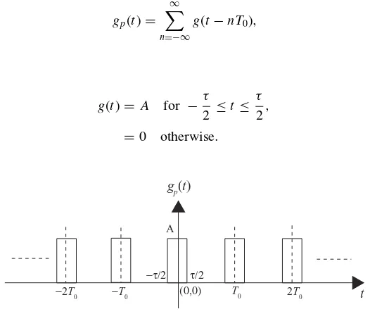
Example 1.1 Figure 1.5 shows a periodic signalgp(t), which is expressed as

gp(t)= ∞

n=−∞

g(t₋nT0),

with

g(t)= A for −τ 2 ≤t≤

τ

2, =0 otherwise.

t g_p(t)

A

τ/2 −τ/2

(0,0) T₀ 2T₀

−T₀

−2T₀

(38)

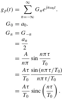
The Fourier series coefﬁcients ofgp(t) in terms of these three representations can be

computed as the following equations show:

(39)

FOURIER SERIES REPRESENTATION OF PERIODIC SIGNALS 9

3. From Eq. (1.12)

gp(t)= ∞

n=−∞

Gnej nω0t.

G0=a0. Gn =G−n

= an 2

= A

nπ sin nπ τ

T0

= Aτ

T0

sin (nπ τ/T0) nπ τ/T0

= Aτ

T0

sinc

nτ T0

.

Figure 1.6 displays theGnfor the case whenA=1 andτ =T0 / 2. Notice that

the Fourier series coefﬁcients of{Gn}are discrete and the dashed line represents the

envelope of{Gn}.

G n

−3 −7

−5 5

3 7

1/2

n 0 1

−1

FIGURE 1.6 Fourier series coefﬁcients of a periodic pulse.

Example 1.2 Let the periodic signalgp(t) in Example 1.1 be modiﬁed withτ =0

andA_{= ∞}, such thatAτ ₌1:

gp(t)= ∞

n=−∞

g(t₋nT0)

= ∞

n=−∞

(40)

(41)

NONPERIODIC SIGNAL REPRESENTATION BY FOURIER TRANSFORM 11

1.4 NONPERIODIC SIGNAL REPRESENTATION BY FOURIER TRANSFORM

A periodic signalgp(t) can always be represented in one of the three Fourier series

forms described in the previous section. Consider the signal based on exponential representation as shown in Eq. (1.12a), that is

gp(t)= ∞

n=−∞

Gnej nω0t,

whereGncan be derived as

(42)

From the integration shown above, it can be seen thatT0Gn is a function ofnω;

therefore, one can deﬁne

(43)

Equations (1.13) and (1.14) are referred to as theFourier transform pair.G(ω) in Eq. (1.14) is considered as the direct Fourier transform of g(t), while g(t) in Eq. (1.13) is the inverse Fourier transform ofG(ω). The transform pair can also be expressed as

G(ω)=F_[g(t)]

and

g(t)=F−1_[G(ω)].

The Fourier transform pair can also be expressed symbolically as

g(t)↔G(ω).

Some key properties of the Fourier transform are listed below:

1. G(−ω)=G∗

(ω) (1.15)

where the asterisk (*) denotescomplex conjugate of. 2. Ifg(t)↔G(ω), then

G(t)↔2πg(−ω). (1.16)

3. g(at)↔ 1 |a|G

ω

a

. (1.17)

4. g(t−t0)↔G(ω)e−jωt0. (1.18)

5. g(t)ejω0t _↔_G₍_ω₋_ω

0). (1.19)

6. Ifg1(t)↔G1(ω) andg2(t)↔G2(ω), then

g1(t)∗g2(t)↔G1(ω)G2(ω), (1.20)

where the asterisk denotes convolution. 7. Ifg1(t)↔G1(ω) andg2(t)↔G2(ω), then

g1(t)g2(t)↔

1

2πG1(ω)∗G2(ω). (1.21)

(44)

Example 1.3 Letg(t) be deﬁned as

g(t)=1 for −τ

2 ≤t ≤

τ

2,

=0 otherwise.

The Fourier transform ofg(t) can be computed as

G(ω)=F_[_g₍_t_)]

=

∞

−∞

g(t)e−jωt_dt

=

τ/2

−τ/2

e−jωt_dt

=τsin ωτ/2 ωτ/2

=τsinc (ωτ/2π).

Figure 1.7 displays the time domain functiong(t) and its Fourier transformG(ω).

g(t)

t

1

τ/2 −τ/2

(0,0)

G(ω)

ω

(0,0) τ

4π/τ 2π/τ 6π/τ −4π/τ

−2π/τ −6π/τ

FIGURE 1.7 A single pulseg(t) and its Fourier transformG(ω).

By comparing Figs. 1.6 and 1.7, one can see that the Fourier series coefﬁcients of a periodic pulse train is the discrete version of the Fourier transform of a single pulse.

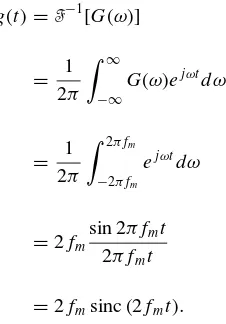
Example 1.4 LetG(ω) be deﬁned as

G(ω)=1 for −2πfm≤ω≤2πfm,

(45)

The inverse Fourier transform ofG(ω) can be computed as

g(t)=F−1_[_G₍_ω_)]

= 1

2π

∞

−∞

G(ω)ejωt_d_ω

= 1 2π

2πfm

−2πfm

ejωtdω

=2fm

sin 2πfmt

2πfmt

=2fmsinc (2fmt).

Figure 1.8 displays the frequency domain functionG(ω) and its inverse Fourier transformg(t).

g(t)

t 1

(0,0)

G(ω)

ω (0,0)

−2πfm 2πfm

2fm

−1/fm

−3/2f_m −1/2fm 1/2fm 3/2fm

1/fm

−2/fm 2/fm

FIGURE 1.8 A single-pulse frequency spectrumG(ω) and its inverse Fourier transformg(t).

Example 1.5 Letg(t)=δ(t), the Fourier transform ofg(t) can be computed as

G(ω)=F_[g(t)]

=

∞

−∞

g(t)e−jωtdt

=

∞

−∞

δ(t)e−jωtdt

(46)

Therefore,δ(t) and 1 are a Fourier transform pair:

δ(t)↔1.

Similarly, ifG(ω)=δ(ω), then

g(t)=F−1_[_G₍_ω_)]

= 1

2π

∞

−∞

δ(ω)ejωtdω

= 1 2π.

Therefore, 1 and 2π δ(ω) are a Fourier transform pair:

1↔2π δ(ω).

1.5 FOURIER TRANSFORM OF A PERIODIC SIGNAL

Although the Fourier transform was derived from the nonperiodic signal, it can also be used to represent the periodic signal. The Fourier transform of a periodic sig-nal can be computed by ﬁrst representing the periodic sigsig-nal in terms of a Fourier series expression, then transforming each Fourier series coefﬁcient (represented in exponential form) into the frequency domain. The following examples illustrate the Fourier transform of periodic signals.

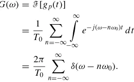
Example 1.6 Letgp(t) be a periodic impulse train, expressed as

gp(t)= ∞

n=−∞

δ(t₋nT0).

The Fourier transform ofgp(t) can be computed by ﬁrst expressing the periodic signal gp(t) in terms of the Fourier series in the exponential form. Thus, from Example 1.2,

we obtain

gp(t)= ∞

n=−∞

Gnej nω0t

= 1

T0 ∞

(47)

FOURIER TRANSFORM OF A PERIODIC SIGNAL 17

whereω0=2π/T0. From Example 1.5, the Fourier transform ofgp(t) can then be

computed as

G(ω)=F_[_g_p₍_t_)]

= 1 T0

∞

n=−∞ ∞

−∞

e−j(ω−nω0)t_dt

= 2π

T0 ∞

n=−∞

δ(ω₋nω0).

Figure 1.9 displays the time-domain impulse traingp(t) and its Fourier transform G(ω). Bothgp(t) andG(ω) appear to be impulse trains. Notice that the amplitude of

the impulse train in the frequency domain isω0and its spectrum repeated at±nω0

withn₌1,2,. . .andω0=2π/T0.

1

t gp(t)

T₀ (0,0)

G(ω)

ω

ω₀

−2ω₀ −ω₀ (0,0) ω₀ 2ω₀

FIGURE 1.9 A periodic impulse train and its Fourier transform.

Example 1.7 Consider the signalgp(t) shown in Example 1.1, expressed as

gp(t)= ∞

n=−∞

g(t₋nT0),

where

g(t)= A for −τ 2 ≤t≤

τ

2, =0 otherwise.

The Fourier transform of the periodic pulse traingp(t) can be computed in two

steps:

Step 1 A periodic signal should ﬁrst be expressed in terms of the Fourier series in exponential form:

gp(t)= ∞

n=−∞

(48)

The Fourier series coefﬁcientsGncan be computed as

G0=

Step 2 The Fourier transform ofgp(t) can then be computed as

G(ω)=F_[gp(t)]

Example 1.5 has shown that

(49)

SAMPLING THEORY AND INTERPOLATION 19

G(ω)

ω −ω₀

−3ω₀ −7ω0

−5ω₀ ω0 5ω0

3ω₀ 7ω0

π

FIGURE 1.10 Fourier transform of a periodic pulse train.

Notice thatG(ω) is a discrete signal that exists whenω=nω0withnequal to an

integer. Figure 1.10 demonstrates the frequency spectrum ofG(ω) forn= −8 to 8, and its envelope is shown as sinc (n/2).

Note that from Figs. 1.6 and 1.10, for the same periodic sequencegp(t), the

am-plitude of Fourier series coefﬁcientsGnand the amplitude of Fourier transformG(ω)

are the same with a scaling difference of only 2π.

1.6 SAMPLING THEORY AND INTERPOLATION

The sampling theory states that any signal that is frequency band-limited tofmcan

be reconstructed from samples taken at a uniform time interval of Ts ≤ 1/(2fm).

The time intervalTs=1/(2fm) is called theNyquist interval, and the corresponding

sampling rate is known as theNyquist rate. The sampling theory can be derived as explained below.

Consider a signalx(t) with its Fourier transform asX(ω) and its frequency spec-trum band-limited tofm. Letgp(t) be a unit impulse train as described in Example

1.6. Multiplication ofx(t) withgp(t) yields the sampled signalxs(t): xs(t)=x(t)gp(t)

=x(t) ∞

n=−∞

δ(t₋nTs). (1.22)

As shown in Example 1.6, a periodic pulse train can be expressed in terms of the Fourier series; that is, withωs=2π/Ts, are obtains

xs(t)=x(t)

1

Ts ∞

n=−∞ ej nωst

= 1

Ts ∞

n=−∞

(50)

FIGURE 1.11 Graphical representations of the sampling theory.

By taking the Fourier transform ofxs(t), one obtains

Xs(ω)=

This equation states that after multiplication ofx(t) by the unit impulse traingp(t),

the new frequency spectraXs(ω) consists ofX(ω), plus replica located atω= ±nωs,

forn₌0,1,2,. . .. The amplitude ofXs(ω) is attenuated by a factor of 1/Ts.

Figure 1.11 illustrates the sampling theory. The original signalx(t) and its analog frequency spectrum_|X(ω)_|are shown in Figs. 1.11a and 1.11b. A periodic impulse traingp(t) and its spectra are shown in Figs. 1.11c and 1.11d. By multiplyingx(t) with gp(t), one can then display the resultantxs(t) in Fig. 1.11e with the corresponding

spectra shown in Fig. 1.11f.

From Fig. 1.11f, one can see that to prevent overlap between the neighboring spectra, the sampling frequencyωs=2π/Tsmust satisfy the requirement thatωs≥

(2×2πfm)=2ωm.

To reconstruct the original signalx(t) from the digitized signalxs(t), one needs to

ﬁlter out the spectrumX(ω), as shown in Fig. 1.11b, from the spectraXs(ω), as shown

in Fig. 2.11f. A lowpass ﬁlter (LPF) with a cutoff frequency at 2πfmand a gain equal

toTsmeets the ﬁltering requirement. By passing thexs(t) through this lowpass ﬁlter,

(51)

SAMPLING THEORY AND INTERPOLATION 21

LettingH(ω) be such a rectangular LPF, one can compute the time-domain func-tionh(t) as

h(t)= 1

2π

2πfm −2πfm

Tsejωtdω

=2fmTs

sin (2πfmt)

2πfmt .

Let the sampling frequencyfs=2fm; then

h(t)=sinc (2fmt). (1.24)

In the time domain, passing the signalxs(t) through the ﬁlterh(t) is equivalent to

havingxs(t) convolved withh(t):

x(t)=xs(t)∗h(t)

=

x(t) ∞

n=−∞

δ(t−nTs) ∗h(t)

= ∞

n=−∞

x(nTs)δ(t−nTs)∗sinc (2fmt)

= ∞

n=−∞

x(nTs) sinc (2fmt−2fmnTs)

= ∞

n=−∞

x(nTs) sinc (2fmt−n). (1.25)

Equation (1.25) states that x(t) can be reconstructed from its discrete samples

x(nTs) and the interpolation function sinc (2fmt –n). Notice thatx(nTs) are all equally

spaced with time intervalTsfor integersn= −∞to∞,and also thatx(t) is a

con-tinuous function in the time domain. Thus, Eq. (1.25) can be used to ﬁndx(t1),for t1=nTs+Tswith <1, based on the discrete values ofx(nTs). The new discrete

time sequencex(t1) can be considered as a resampling ofx(t), or interpolated from x(nTs).

In practical applications, the resampling process that utilizes the interpolation fil-ter sinc (2fmt) is simplified by two approximations. First, the interpolation filter is

(52)

FIGURE 1.12 Interpolation ﬁlters.

image processing. This set of 16 sinc ﬁlters provides a fractional sample shift from

1

16 =1 is not considered a sample shift.

Figure 1.12 displays the waveforms of 16 sets of interpolation filters with each having 8-tap coefficients. Figure 1.12a shows a reference sinc (t) function with 5 sidelobes around the mainlobe. The window function is normally applied to the inter-polation filter, yet no window or rectangular window is used here for simplification. Figure 1.12b displays four interpolation filters with delays equal to ₁₆1,₁₆5,₁₆9, and13₁₆ sample intervals with respect to the top reference function, respectively. Figure 1.12c displays the digitized version of all 16 interpolation filters, and each one corresponds to a ₁₆1 sample delay from each other.

Table 1.1 lists the coefficients of the 16 interpolation filters, with each one having 8 coefficients. The first row of filters has a shift of ₁₆1 sample interval, while the last one has 16₁₆ =1 or no sample shift. From Table 1.1 and Fig. 1.12c, one can see that the interpolation filters are symmetric; that is, filter coefficients of row 1 with ₁₆1 sample shift are the same as that of row 15 with15₁₆ sample shift, except that they are time-reversed. The filter coefficients of rows 1, 5, 9, and 13 of Table1.1 correspond to the four sinc filters shown in Fig. 1.12b.

To illustrate the principle of resampling based on an interpolation ﬁlter, consider a signalx(n) that consists of three normalized frequencies,f1=0.15,f2=0.25, and f3=0.45, and is expressed as

x(n)=0.35 cos (2πn f1)+0.2 sin (2πn f2)−0.4 cos (2πn f3),