Manajemen | Fakultas Ekonomi Universitas Maritim Raja Ali Haji 073500102288618829

Full Terms & Conditions of access and use can be found at

http://www.tandfonline.com/action/journalInformation?journalCode=ubes20

Download by: [Universitas Maritim Raja Ali Haji] Date: 13 January 2016, At: 00:39

Journal of Business & Economic Statistics

ISSN: 0735-0015 (Print) 1537-2707 (Online) Journal homepage: http://www.tandfonline.com/loi/ubes20

Indirect Inference, Nuisance Parameter, and

Threshold Moving Average Models

Alain Guay & Olivier Scaillet

To cite this article: Alain Guay & Olivier Scaillet (2003) Indirect Inference, Nuisance Parameter, and Threshold Moving Average Models, Journal of Business & Economic Statistics, 21:1, 122-132, DOI: 10.1198/073500102288618829

To link to this article: http://dx.doi.org/10.1198/073500102288618829

View supplementary material

Published online: 01 Jan 2012.

Submit your article to this journal

Article views: 54

View related articles

Indirect Inference, Nuisance Parameter, and

Threshold Moving Average Models

Alain

Guay

Département des Sciences Economiques, Université du Québec à Montréal and CIRPÉE, Montréal, P.Q. H3C 3P8, Canada (guay.alain@uqam.ca)

Olivier

Scaillet

HEC Genève and FAME (olivier.scaillet@hec.unige.ch)

We analyze the modiŽcations that occur in indirect inference when a nuisance parameter is not identiŽed under the null hypothesis. We develop a testing procedure adapted to this simulation-based estimation method, and detail its use for detecting the threshold effect in threshold moving average models with contemporaneous and lagged asymmetries. In contrast to existing threshold models, these models allow taking into account the presence of asymmetric effects of current and lagged random shocks. We use them to measure the persistence of shocks to U.S. output.

KEY WORDS: Asymmetric time series; GNP analysis;p-value transformation; Shock persistence; Simulation-based inference.

1. INTRODUCTION

This article considers inference when a nuisance parame-ter is not identiŽed under the null hypothesis in the context of simulation-based econometric methods. Simulation-based econometric methods are increasingly used in economics and Žnance for models which were previously thought to be too complex for a proper estimation. The reason is that they allow the estimation of models where the optimizing function takes no simple analytical form. In such models, the difŽculty may, for example, arise from the presence of multidimentional inte-grals in the likelihood function or in the moment conditions. In this context, conventional econometric methods cannot be directly used since they require an explicit form for the opti-mizing function. Simulation-based econometric methods are designed to overcome such a numerical difŽculty through an approach based on simulated data. The only requirement to implement these indirect methods is that the model can be simulated. They include the simulated method of moments (DufŽe and Singleton 1993), indirect inference (Gouriéroux, Monfort, and Renault 1993), and the efŽcient method of moments (Gallant and Tauchen 1996).

In this article, we examine the problem occurring when a nuisance parameter is not identiŽed under the null in the context of indirect estimation methods. This problem is well studied in the direct estimation context [see Andrews and Ploberger (1994), Hansen (1996), among others]. Indirect esti-mation methods are characterized by the use of an auxiliary model and simulation paths from the structural model. The purpose of our article is to analyze the problem of a nuisance parameter, which is not identiŽed under the null in this setup. In the case of structural change tests with unknown break-point, Ghysels and Guay (2001a,b) show, for simulation-based estimation methods, that the asymptotic distribution of stan-dard tests is free of nuisance parameters. In that setting, the parameter that appears under the alternative, but not under the null, is the time of structural change. However, the asymp-totic distribution of standard tests generally depends upon unknown parameters. In this article, we analyze the modiŽ-cations that occur in indirect methods in the general case. To

do so, we modify the strategy proposed by Hansen (1996) in the direct estimation context. In particular, we show how to deal with inference when additional uncertainty is intro-duced due to simulations. The general framework is developed for estimation by indirect inference. As shown by Gouriéroux and Monfort (1995a), indirect inference contains the simu-lated method of moments (SMM) and the efŽcient method of moments (EMM) as special cases. The results derived in this article are thus directly applicable to these methods.

The general setting is applied to threshold moving average (TMA) models in the context of an analysis of the persis-tence of shocks to output. By relaxing the hypothesis of sym-metry, Beaudry and Koop (1993) and Elwood (1998) allow the disentanglement of effects of positive shocks versus neg-ative shocks. Beaudry and Koop (1993) use an exogenous proxy to represent shocks, and provide evidence of asymmet-ric effects of innovations to the gross national product (GNP) [see Elwood (1998) for a critic of the speciŽcation used by Beaudry and Koop (1993) to identify positive and negative shocks]. Negative shocks to GNP seem to be less persistent than positive shocks. In contrast to Beaudry and Koop (1993), Elwood (1998) identiŽes directly positive and negative shocks by using an unobserved component model corresponding to a threshold moving average model. He Žnds no evidence of asymmetry in the persistence of shocks to output. However, his modeling excludes an a priori asymmetric effect of con-temporaneous shocks, and imposes a threshold depending on the sign of shocks.

In this article, we consider a more exible model to analyze the persistence of shocks to output. This model takes the form of the following threshold moving average model [TMA(l)]:

Y_tDŒCd₀C…_{t …t>ƒ}Cdƒ₀…_{t …tµƒ}

C¢ ¢ ¢CdlC…tƒl …tƒl>ƒCd

ƒ

l …tƒl …tƒlµƒ (1)

©2003 American Statistical Association Journal of Business & Economic Statistics January 2003, Vol. 21, No. 1 DOI 10.1198/073500102288618829

122

where A takes the value 1 if A is true and 0 otherwise. In

model (1), successive shocks are not transmitted symmetri-cally through time, but their inuence does depend on their exceedance of the threshold ƒ. The main feature of model (1) is thus its ability to capture asymmetric effects induced by the random shocks. As opposed to Elwood (1998), we do not impose a threshold value, and we introduce contempora-neous asymmetry. Such an asymmetry, if present, will affect the measurement of persistence of shocks.

Threshold moving average (TMA) models have already been considered in Tong (1990), but without any contem-poraneous asymmetry [see also related work by Wecker (1981) and De Gooijer (1998)]. This extension parallels the construction proposed for the conditional variance by El Babsiri and Zako¨õan (2001) in a generalized

autore-gressive conditional heteroscedastic (GARCH) context. The contemporaneous asymmetry induces second moments, which differ depending on the threshold. The introduction of the contemporaneous asymmetry in model (1) prevents a direct approach by maximum likelihood. Therefore, we need to pro-ceed by indirect methods to estimate the parameters of this type of TMA model.

In empirical work, the presence of contemporaneous and lagged asymmetries needs testing. The inference is not stan-dard because a nuisance parameter (the threshold) is not iden-tiŽed under the null hypothesis. We apply the general results developed in the Žrst part of the article to test for the presence of asymmetry in the moving average representation.

The article is organized as follows. In Section 2, we present the general framework and testing problem. The setting is suf-Žciently large to cover a broad category of dynamic models. In Section 3, we describe how to accommodate the indirect infer-ence procedure of Gouriéroux, Monfort, and Renault (1993) in the presence of a nuisance parameter. The general frame-work and results are then applied to TMA models in Section 4. Properties, estimation, and tests for such models are therein detailed, the threshold being the nuisance parameter. Some Monte Carlo results are also proposed. An empirical applica-tion is delivered in Secapplica-tion 5, and consists of an analysis of the persistence of shocks to U.S. GNP growth rates. Section 6 contains some concluding remarks. All proofs are gathered in the Appendix. The usual notational conventions are used in the article.˜¢˜ denotes the Euclidean norm of a vector or a matrix,˜¢˜r denotes theLr norm of a random vector, that is,

˜X˜rD4E˜X˜r₅1=r_{, and the symbol)denotes weak}

conver-gence as deŽned in Pollard (1994).

2. GENERAL FRAMEWORK AND TESTING PROBLEM

We consider a multivariate stationary process:wtD4yt01 x0t50

wherey_t is aG-dimensional vector andx_t is aK-dimensional vector. We assume that the true conditional pdf of w_t given w_tƒ1 D 8wtƒ11 wtƒ21 : : : 1 9 (w.r.t. some measure )

only depends on w_tƒ11 : : : 1 wtƒk, for some k. This pdf is

denoted f04wt—wtƒ15, and can be written as f04wt—wtƒ15D

f0y4yt—xt1 wtƒ15f0x4xt—xtƒ15, where f0y and f0x are pdf w.r.t.

some measuresŒx andŒy, respectively.

We are interested in modeling f0y, and consider M D 8f 4yt—xt1 wtƒ13 ˆ1 ƒ51 ˆ 2ä1 ƒ 2 â 9, a parametric family of

pdf, whereä andâ are compact and bounded subsets ofRq andRm, respectively. In short,Mis a parametric model for the conditional distribution of the processyt given the processxt,

where ˆ will be the parameter of interest and ƒ the nuisance parameter. The parameterˆ is decomposed intoˆD4ˆ011 ˆ0250,

whereˆ12Rq1,ˆ22Rq2, andqDq1Cq2. For notational

con-venience,f 4yt—x_t1 w_tƒ13 ˆ1 ƒ5is denoted hereafter asf_t4ˆ1 ƒ5. Our testing problem can be described as follows. The null hypothesis is

H₀2 8ˆ₂D09 while the alternative hypothesis is

H12 8ˆ26D091and the modelM depends on the parameterƒ0

We let ˆ₀ denote a parameter vector in the null hypothe-sis. Under the null, we assume that f0yDft4ˆ01 ƒ5 does not

depend on the parameterƒ. The parameterƒ is not identiŽed under the null, and has to be treated as a nuisance parame-ter. The testing procedure is therefore not standard as we treat ƒ as unknown. As usual, in this setting, we adopt a local-to-null reparameterization ˆ₂Dc=pT, and the null hypothesis becomesH02 8cD09.

3. INDIRECT INFERENCE WITH NUISANCE PARAMETER

We consider a situation where maximum likelihood esti-mation or estiesti-mation by a method of moments are not fea-sible, and an indirect procedure is called for. Indeed, maxi-mum likelihood estimators are not always available, and one should then rely on auxiliary or instrumental models through indirect procedures. The terminology auxiliary model versus instrumental model can be used interchangeably [see Dhaene, Gouriéroux, and Scaillet (1998) for interpretation]. We mod-ify here the results of Hansen (1996) to account for this indi-rect estimation, and derive the asymptotic distribution theory underH₀2 8cD09. In the following, we sketch briey the indi-rect inference procedure, and refer the reader to Gouriéroux, Monfort and Renault (1993) and Gouriéroux and Monfort (1995a) for details [see also Smith (1993)]. As already pointed out, SMM and EMM can be viewed as particular cases of indirect inference.

Let us assume that we can draw freely some paths from the conditional model for a given value of the parameters. We denote byyn

t4ˆ1 ƒ5,tD11 : : : 1 T,nD11 : : : 1 N, the

com-ponents of the N drawn paths. To assist us in the estima-tion, we choose an instrumental criterion characterized by QT4yT—xT1 wTƒ13 ‚5DPTtD1qt4yt—xt1 wtƒ13 ‚5,‚2B withB a

compact subset ofRp _{andp¶q. This criterion may, for}

exam-ple, correspond to a likelihood function. Further, let us intro-duce theM-estimators of‚:

O

‚_T Darg min

‚2B

Q_T4y_T—x_T1 w_Tƒ13 ‚5

and

computed from the data and the simulated values, respectively. The binding function b4ˆ1 ƒ5, for a given value of ƒ, will be the limiting value of ‚ON_{4ˆ1 ƒ5 (Gouriéroux and Monfort}

1995a). Under the null, the binding function does not depend on the parameterƒ, and is denoted‚0Db4ˆ05. The indirect

where ìb_T4ƒ5 is a positive-deŽnite matrix converging to a deterministic positive matrixì4ƒ5for a Žxedƒ. Optimal indi-rect estimators are obtained with a weighting matrix corre-sponding to an estimator ofìü_{4ƒ5deŽned below in}

assump-tion (p).

The scores associated with the instrumental model are denoted by

some neighborhood ofˆ0.

(d) ‚ON

T4ˆ1 ƒ5is continuously partially differentiable inˆfor

allˆ2ä0 andƒ2â with probability 1 under the null.

(e) b4ˆ1 ƒ5is continuously partially differentiable inˆ for allˆ2ä0 andƒ2â.

(h) qt4‚5is twice continuously partially differentiable in‚

for all‚2B0 with probability 1 under the null, where B0 is

some neighborhood of‚0.

(i) qn

t4‚1 ˆ1 ƒ5is twice continuously partially differentiable

in‚for all‚2B0,ˆ2ä0 andƒ2â with probability 1 under

and ‚ 2B0 under the null for some nonrandom function

Jq4‚1 ƒ5uniformly continuous in4‚1 ƒ5overB0€â.

and for some nonrandom function Jq4b4ˆ1 ƒ51 ƒ5 uniformly

continuous in4b4ˆ1 ƒ51 ƒ5overä0€â.

(l) Jq4‚01 ƒ5is uniformly positive deŽnite overƒ2â.

(m) Tƒ1=2PT

tD1sq1 t4‚05 H) Sq4‚01¢5 under the null as Gaussian processes indexed by ƒ 2â with mean zero and covariance matrixIq4‚01¢5.

(n) Tƒ1=2PT

tD1sq1 tn 4‚01 ˆ01¢5H)Sqn4‚01¢5under the null as Gaussian processes indexed by ƒ 2â with mean zero and covariance matrixIq4‚01¢5.

Assumption (a) gives an indirect estimator, which does not depend on the nuisance parameter under the null. Assump-tions (b)–(g) are classical in indirect inference, and are only slightly modiŽed to handle the presence of a nuisance param-eter. They concern the behavior of the estimators and their limits. In particular, the injectivity of the binding function and the rank condition on its derivative embodied by assumption (g) are global and local identiŽability conditions for indirect inference (Dhaene, Gouriéroux, and Scaillet 1998). Note that we only require differentiability w.r.t. the parameter of inter-est ˆ, and not w.r.t. the nuisance parameterƒ. Assumptions (h), (i), (k), and (l) are standard in the context of M esti-mation. In assumption (j), the probability limit of the score function for the data is indexed by the nuisance parameterƒ since the derivative of the limit criterion of the instrumental depends on ˆ andƒ [see Gouriéroux, Monfort, and Renault (1993)]. Assumptions (m) and (n) are relative to the weak con-vergence of the score functions. In particular, assumption (n) corresponds to the score of theM estimator for the simulated pathn. Assumptions (o) and (p) on the weighting matrix lead to optimal indirect estimators.

The Wald statisticWT4ƒ5for the null hypothesisH02 8cD

09is given by

The score statistic is the gradient of the objective function w.r.t. ˆ evaluated at the constrained estimatorˆQN

T obtained by

where VeT4ƒ5 is the variance-covariance matrix ofCT4ƒ5 [see

Gouriéroux, Monfort, and Renault (1993) for the expression of this matrix].

Finally, the LR-type test is based on the difference of the optimal values of the objective function for the constrained and unconstrained estimators:

The following theorem gives the asymptotic distribution of the concentrated indirect estimator and theW_T4ƒ5, LM_T4ƒ5, andLR_T4ƒ5 statistics.

Theorem 1. UnderH₀2 8cD09 and Assumption 1,

The asymptotic distribution of WT4ƒ51 LMT4ƒ5, and LRT4ƒ5statistics is a chi-square distribution for a givenƒ. For ƒ2â, one can then build statistics such asg4WT4ƒ55, where g maps functionals onâ toR. Davis (1977, 1987) suggested using the supremum (Sup), and Andrews and Ploberger (1994) show that superior local power can be obtained by the average (Ave) of the statistics onâ or by an exponential transforma-tion. However, the asymptotic null distribution of these map-pings depends in general on the true parameter valueˆ0, and

critical values cannot be tabulated.

Hansen (1996) proposes a nice remedy, namely, a p-value transformation, based on a simple simulation technique in order to obtain empirical estimates of asymptotic p val-ues. His methodology can be easily adapted to our frame-work. It consists of working conditionally on the sample and simulated paths and using iid N 40115 draws to build conditional mean zero Gaussian processes with appropriate second-moment characteristics. Let vt, vtn, nD11 : : : N, be NC1 independent standard normal variables. We set bSq1 T D

Tƒ1=2PT

q1 t4ƒ5 denote the estimates of the scores. The

differ-ence between direct and indirect estimation lies in the pres-ence of theN estimates of the scores corresponding to theN simulated paths. The four steps described in Hansen (1996) can then be performed by using SSN

q1 T4ƒ5DJq1 T4ƒ5ƒ14bSq1 Tƒ

1

N

PN

nD1bSq1 Tn 4ƒ55 at the second step, and the Žnite sample

statistic corresponding to the asymptotic distribution of the tests statistic (Theorem 1) at the third step to obtain the empir-ical p values. Since we operate conditionally on the sample and the simulated paths, all randomness appears in the iid vari-ablesvtandvtn,nD11 : : : 1 N. Therefore, as in Hansen (1996),

we may conclude that bS_{q1 T} and bSn

q1 T4¢5 converge weakly in probability to S_q4‚01¢5 and Sqn4‚01¢5, respectively, as Gaus-sian processes indexed byƒ2â with mean zero and covari-ance matrix Iq4‚01¢5. By the Glivenko–Cantelli theorem, the simulated p values converge in probability to the true one. It is important to note that the asymptotic covariance matrix

S

Vq4‚01 ƒ5 is scaled by a factor 41C1=N 5, which contrasts

with the direct estimation case. This scale factor depends on the number of simulated paths. In Section 4.2, a small sample study examines the impact of the number of simulated paths on the estimation and testing properties for our application.

4. THRESHOLD MOVING AVERAGE MODELS In this section, we outline the threshold moving average model which will be used in the empirical section to measure asymmetry in the persistence of shocks to output. Basic prop-erties of this model are presented before developing estimation and testing strategies.

Testing procedures involving a nuisance parameter have already been used to detect a threshold effect in threshold autoregressive models [see, e.g., Chan (1990), Hansen (1996)] or parameter instability [see, e.g., Andrews (1993), Andrews and Ploberger (1994), Ghysels, Guay, and Hall (1998), Ghysels and Guay (2001a,b), and Sowell (1996)]. In this arti-cle, we want to study the threshold model:

YtDŒCDC4L5…Ct CDƒ4L5…ƒt (2)

with …C

t D…t …t>ƒ, …

ƒ

t D…t …tµƒ, and …t ¹ iid N 40115. The

nuisance parameter ƒ corresponds to the threshold govern-ing the asymmetric effects of the random shocks. The poly-nomials of order l 2 DC_{4L5 Dd}C

0 Cd1CLC¢ ¢ ¢CdlCLl and Dƒ_{4L5 D d}ƒ

0 Cdƒ1LC¢ ¢ ¢CdlƒLl drive the moving

aver-age dynamics of the error term. The introduction of dC0

and d₀ƒ leads to the presence of a contemporaneous asym-metry [see Zako¨õan (1994) for ARCH asymmetries and

El Babsiri and Zako¨õan (2001) for similar contemporaneity

in the conditional variance]. The parameter of interest ˆD 4Œ1 d0C1 dC11 : : : 1 dCl1 d0ƒ1 dƒ11 : : : 1 dlƒ50 is made of the mean

and the coefŽcients of the moving average polynomials. Wecker (1981) proposes asymmetric moving average mod-els with a threshold depending on the error term, but the case with contemporaneous asymmetry is not considered, and the threshold is arbitrarily Žxed to zero. Elwood (1998) employs the asymmetric moving average model proposed by Wecker to study the asymmetry in the persistence of shocks to output. In

contrast to Elwood, we allow for contemporaneous asymme-try, and we do not restrict the threshold to be equal to zero. In the following, we describe how to estimate asymmetric mov-ing average models with contemporaneous asymmetry, and how to test the presence of asymmetry without a priori impos-ing the value of the threshold. De Gooijer (1998) also con-siders threshold moving average models with a contempora-neous effect. However, his threshold depends on the observed variable [self-exciting threshold moving average (SETMA) models].

Let us Žrst examine the basic features of model (2) before moving to the estimation and testing procedures.

4.1 Basic Properties

In model (2), the conditional distribution of Yt is a mixture

of the distributions of…C_t and…_tƒ. This will lead to skewed and leptokurtic (or platykurtic) conditional distributions. To quan-tify this effect, one needs to deŽne an information set to yield truly iid errors. The required information set must include past values of…t. Indeed, the information set including only past

values of the observed process is not sufŽcient to obtain iid errors. The required information set at timetƒ11 I_tƒ1 is then deŽned as Itƒ1D8…tƒ19. Let us introduce the strong

inno-vation process Ut of Yt, deŽned by UtDYtƒE6Yt—…tƒ17D

d₀C‡C

t Cdƒ0‡ƒt , where‡Ct D…tCƒE6…Ct 7, and‡ƒt D…ƒt ƒE6…ƒt 7

are iid centered processes, independent of the past, and where d0C anddƒ0 are the Žrst coefŽcients of the polynomialsDC4L5

andDƒ4L5.

Proposition 1. In model (2) when ƒD0, the conditional skewness ofYt is given by

E6U_t3—…_tƒ17

E6U2

t—…tƒ173=2

D64d C

053ƒ4dƒ05374C25C364d0C52d0ƒƒd0C4dƒ05274ƒ25

£

64dC₀52_C4dƒ

05274ƒ15C2dC0d0ƒ

¤3=2

and the conditional kurtosis ofY_t by

E6Ut4—…tƒ17

E6U2

t—…tƒ172

D

64dC₀54_C4dƒ

0547462ƒ10ƒ35C464d0C53d0ƒCd0C4dƒ0537

€4C35C64d0C524dƒ05242ƒ35

£

64d₀C52_C4dƒ

05274ƒ15C2dC0dƒ0

¤2 0

Proposition 1 gives the conditional skewness and kurtosis ofY_t when the thresholdƒ is equal to zero. Expressions for anyƒcan also be computed thanks to the general forms given in the Appendix. Eventually, unconditional skewness and kur-tosis can also be derived, but the computations involve tedious algebra. The conditional moments w.r.t. the information set Iü

tƒ1DYtƒ1can be computed by simulations. The marginal and

conditional skewness and kurtosis ofY based on the informa-tion setI_tƒ14Itƒ1 Itƒü15will imply marginal and conditional

skewness and kurtosis ofY based on the information setIü tƒ1.

The next proposition is related to the autocovariance struc-ture of a TMA4l5model withƒD0.

Proposition 2. In a threshold moving average model with llags andƒD0, the autocovariancesƒ4u5N are given by

N ƒ4u5D

lƒu

X

iD0

³

4d_iCuC d_iCCd_iCuƒ dƒ_i 5ƒ1 2

C4dC_iCudƒ_i Cd_iCuƒ dC_i5 1 2

´

1 uµl

D01 u > l0

From this proposition, it transpires that the autocorrelation function (ACF)84u5D Nƒ4u5=ƒ4N 053 uD1121 : : : 9of a series following a TMA4l5model is zero for lagsu > l. Thus, it will be difŽcult to separate this model from an MA4l5 model on the basis of the cutoff point of the sample ACF. Even though second-order features are not relevant to distinguish between TMA4l5 and MA4l5 models, possible skewness and excess kurtosis in the series will lead to favoring the former instead of the latter. The threshold testing procedure developed in the next section will also be of further help in making such a decision.

4.2 Estimation and Tests

The q€1 parameterˆD4Œ1 dC01 d1C1 : : : 1 dlC1 dƒ01 dƒ11 : : : 1

d_lƒ50cannot be estimated by maximum likelihood. Indeed, due to the contemporaneous asymmetry, we cannot adopt a direct approach, and we need to rely on indirect estimation.

We consider here simple linear instrumental models in esti-mation by indirect inference. Indeed, Gouriéroux, Monfort, and Renault (1993) have shown in the case of an MA(1) pro-cess that the indirect inference estimator obtained with an AR(3) instrumental model has good Žnite sample properties, and outperforms the asymptotically most efŽcient estimator. Since a TMA model boils down to a standard MA model under the null, that is, the absence of a threshold effect, we also choose linear autoregressive processes as instrumental models. The Žrst one is a pure linear AR4p5process with the following log-likelihood function:

ƒ4Tƒp5

2 ln 2ƒ 4Tƒp5

2 ln‘

2

ƒ T

X

tDpC1

¡

Y_tƒƒê₁Y_tƒ1ƒ¢ ¢ ¢ƒêpYtƒp

¢2

2‘2 0

This type of instrumental model is particularly appealing since the PML estimator of the parameter ‚D41 ”11 : : : 1

”p1‘25of dimension larger or equal toq corresponds to the

OLS estimator. Regularity conditions concerning the behavior of the binding and score functions are further met (see The-orem 2 below) since the instrumental model is a regression type model, andYttakes a linear form inˆ(a pure MA model

under the null).

The second instrumental model tries to capture nonlinear-ity in the observed process in order to obtain more precise estimates of the parameters of interest. To do so, we intro-duce the second and third polynomials for the lags ofYt in the

AR representation as proposed by Michaelides and Ng (2000).

The log-likelihood function is

ƒ4Tƒ₂p5ln 2ƒ4Tƒ₂p5ln‘2

ƒ

T

X

tDpC1

¡

Ytƒƒê1Ytƒ1ƒê2Yt2ƒ1ƒê3Yt3ƒ1ƒ¢ ¢ ¢ƒê3€pYt3ƒp

¢2

2‘2 0

In order to evaluate the performance of these instrumental models, we execute a simulation study. Two dimensions are of interest in the design of experiments: the order of the AR process and the number of simulated paths.

The model of interest for the simulation study is the fol-lowing threshold moving average model of order 1:

YtDdC0…t …t>0Cd

ƒ

0…t …tµ0

CdC₁…_tƒ1 …tƒ1>0Cd

ƒ

1…tƒ1 …tƒ1µ0 (3)

where the threshold is Žxed to zero, anddC0 D051 d0ƒD11 d1CD

02, and dƒ1 D08. In this representation, the negative shocks

have a stronger impact than the positive ones. The sample size is equal to 200, and the number of replications is 500.

How can we know whether we should take into account a threshold effect in the dynamics of the shocks in model (3)? By writingˆ1D4dC01 dC150ˆ2D4dƒ01 d1ƒ50ƒ4dC01 dC150, we

see that the answer is given by testing the null hypothesis H02 8ˆ2D09. The following theorem justiŽes the application

of results in Section 3 to the model of interest and instrumental models under consideration.

Theorem 2. Under the model of interest and the instru-mental models deŽned above, assumptions (a)–(p) hold. The asymptotic distribution of Wald, LM, and LR statistics is given under the null by Theorem 1, and under the alternative by

p T R04ˆON

T4¢5ƒˆ05H)

¡

ƒR0KS_q4‚01 ˆ01¢5SSqN4‚01¢5

¢

Cc

and

WT4¢51 LMT4¢51 LRT4¢5H)

¡

4R0KSq4‚01 ˆ01¢5SSqN4‚01¢55Cc

¢0

€£

R0SVq4‚01 ˆ01¢5R

¤ƒ1

€¡

4R0KSq4‚01 ˆ01¢5SSqN4‚01¢55Cc

¢

as processes indexed byƒ2â.

Proof. See Appendix.

For the Žrst instrumental model, we consider AR(4), AR(6), AR(8), and AR(10) processes. The results for the bias and the root mean square errors (RMSE’s) are reported in Table 1.

Table 1. Instrumental Model I

AR(4) AR(6) AR(8) AR(10)

Parameters Bias RMSE Bias RMSE Bias RMSE Bias RMSE

dC

0 ƒ00874 02689ƒ00864 02912ƒ01040 03432ƒ00903 03601

dƒ

0 ƒ00964 02523ƒ01037 02943ƒ00871 03171ƒ00915 03417

dC

1 01126 03281 00987 03628 00661 04058 00492 04168

dƒ

1 00360 02611 00255 03022 00125 03484 00008 03759

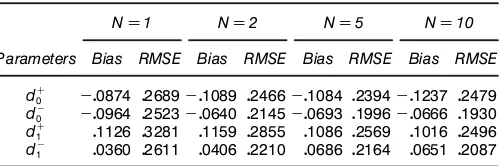
Table 2. Instrumental Model I With AR(4)

ND1 ND2 ND5 ND10

Parameters Bias RMSE Bias RMSE Bias RMSE Bias RMSE

dC

0 ƒ00874 02689ƒ01089 02466ƒ01084 02394ƒ01237 02479

dƒ

0 ƒ00964 02523ƒ00640 02145ƒ00693 01996ƒ00666 01930

dC

1 01126 03281 01159 02855 01086 02569 01016 02496

dƒ

1 00360 02611 00406 02210 00686 02164 00651 02087

We note that the estimates are not very precise. While the increase of the order of the AR process decreases the bias, the extra parameters included in the instrumental model increase the variance of the estimates. Indeed, the smallest RMSE is obtained with an AR(4) process.

Table 2 reports the results for various number of sim-ulated paths with the instrumental model corresponding to an AR(4) process. The precision of the estimates is greatly improved when increasing the number of simulated paths. The bias decreases for the parameters corresponding to the nega-tive shocks. It increases for the parameters corresponding to the positive shocks. The importance of the reduction gain for RMSE appears particularly important for N D2 and N D5. The difference betweenN D5 andND10 is negligible.

The results for instrumental model II are gathered in Table 3. Introducing nonlinearity in the conditional mean decreases the bias for the parameters corresponding to the pos-itive shocks, and slightly increases the bias for the parameters corresponding to the negative shocks. In all cases, the pre-cision of the estimates is signiŽcantly improved. The AR(2) representation seems to give the best results in terms of bias and RMSE.

In conclusion, parsimonious representations give the best results in light of the root mean square error criterion. Accounting for nonlinearity by the introduction of polynomi-als in the autoregressive instrumental model improves the pre-cision of the estimates.

We consider a third instrumental model which is a mix of the two previous instrumental models. The model is the following:

Y_tDê₁Y_tƒ1Cê₂Y_tƒ2₁Cê₃Y_tƒ3₁Cê₄Y_tƒ2Cê₅Y_tƒ2₂

Cê₆Y_tƒ3₂Cê₇Y_tƒ3Cê₈Y_tƒ4C…_t0 This representation includes the speciŽcations which yields the best performance for the Žrst and second instrumental models. Table 4 reports the results for various number of simulated paths. ForN D1, we see that this instrumental model clearly

Table 3. Instrumental Model II

AR(1) AR(2) AR(3) AR(4)

Parameters Bias RMSE Bias RMSE Bias RMSE Bias RMSE

dC

0 ƒ00010 02100ƒ00134 01953 00087 02142 00180 02073

dƒ

0 ƒ01561 02974ƒ00925 02366ƒ01159 02541ƒ01201 02534

dC

1 01373 03938 00104 02238 00147 02468 00286 02360

dƒ

1 00503 02592 00336 02697 00121 02667 00160 02461

Table 4. Instrumental Model III

ND1 ND2 ND5 ND10

Parameters Bias RMSE Bias RMSE Bias RMSE Bias RMSE

d0C ƒ00324 01561ƒ00154 01550ƒ00105 01440ƒ00070 01336

dƒ

0 ƒ00431 01930ƒ00578 01781ƒ00646 01816ƒ00616 01722

d1C 00196 02028 00046 01571ƒ00069 01479ƒ00072 01410

dƒ

1 00118 02142 00204 02077 00270 01937 00161 01874

outperforms the two other instrumental models in terms of RMSE with a large reduction in bias. We observe the same pattern as that of the other instrumental models when the num-ber of simulated paths increases. In conclusion, the bias is small with this instrumental model, and the precision of the estimates is acceptable for a sample of 200 observations.

Let us now perform a simulation study to evaluate the small sample properties of the adaptation of the Hansen (1996) strat-egy to indirect inference. In this assessment of the size and power of the testing procedure, we keep the model given by Equation (3). Under the null, it corresponds to an MA(1) pro-cess. The parameterd0 is Žxed to 1 andd1 to .5, while

sam-ple sizes are equal to 200. Due to the large computational requirements of the simulation design, only 200 simulated samples are generated. The interval for the threshold was set to6ƒ051 057, with evaluation points spaced by .05.

Two mappings of the Wald andLMstatistics are examined: supremum (Sup) and average (Ave). The asymptotic distribu-tion of these statistics under the null is approximated with 500 replications.

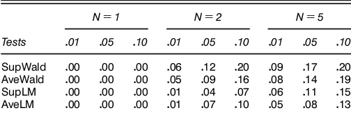
Table 5 contains the results where N equals 1, 2, and 5. For the case of a single simulated path, the estimation is too imprecise. Consequently, the null hypothesis is never rejected. However, the results withN D2 andN D5 are more encour-aging. The functions based on the Wald statistics reject the null too frequently. The functions based on theLM statistics give results close to the corresponding size. In particular, the averageLMstatistic seems to reject the null with accurate size. To evaluate the power of the tests, we consider Equation (3) withd₀CD05,dƒ

0 D1,dC1 D02, anddƒ1 D08, and the threshold

Žxed to zero. Table 6 shows the results. WhenND1, the tests have no power to detect the threshold effects in the MA part. ForN D2, and particularly forND5, the power is very good. For example, the averageLMstatistic rejects the null with a probability of .91 at a size corresponding to .05.

In conclusion, for a sample of 200 observations, the func-tions based on theLMstatistics have good size for a number of simulated paths equal to or greater than 2. Moreover, the power forN equal to or greater than 2 is high and increasing inN.

Table 5. Sample Size of the Tests for 200 Observations

ND1 ND2 ND5

Tests 001 005 010 001 005 010 001 005 010

SupWald 000 000 000 006 012 020 009 017 020

AveWald 000 000 000 005 009 016 008 014 019

SupLM 000 000 000 001 004 007 006 011 015

AveLM 000 000 000 001 007 010 005 008 013

Table 6. Sample Power of the Tests for 200 Observations

ND1 ND2 ND5

Tests 001 005 010 001 005 010 001 005 010

SupWald 000 000 000 055 074 085 086 093 096

AveWald 000 000 000 053 075 085 086 093 095

SupLM 000 001 005 046 061 066 085 091 094

AveLM 001 003 005 048 064 070 084 091 094

5. APPLICATION TO THE PERSISTENCE OF SHOCKS

In this section, we apply the estimation and testing strategies developed in the previous lines to measure the persistence of shocks to the real U.S. GNP growth rate (seasonally adjusted) for the period corresponding to the Žrst quarter of 1947 to the Žrst quarter of 1991. We use this sample to compare our results to the results obtained by Elwood (1998).

To assess the ARMA speciŽcation for the GNP, we exam-ine the autocorrelation and partial autocorrelation functions. The Žrst two autocorrelations and the Žrst partial correlation are signiŽcant. Thus, an AR(1) or an MA(2) process could possibly Žt the series. For the AR(1) process, the residuals are still correlated (thepvalue for the Breusch–Godfrey serial correlation LM test with two lags is equal to .04). In con-trast, the residuals for the MA(2) process are not correlated, whether we look at the Breusch–Godfrey serial correlationLM test (p value equal to .46 with two lags) or the Q statistic (Box–Pierce statistic). Also, the sum of squared residuals is smaller for the MA(2) process compared to that of the AR(1) process. Therefore, the MA(2) model is adopted.

We run a RESET test to detect nonlinearity for the MA(2) process. The null hypothesis of linearity is highly rejected with apvalue equal to .000024. This is conŽrmed by the skewness 4ƒ0155 and excess kurtosis (3.45) of the series. Besides, no ARCH effects are detected on residuals. Hence, a threshold moving average model seems to be an interesting alternative to the traditional moving average model.

To implement the estimation of the TMA model, we need an instrumental model. We choose instrumental model III, including six lags for the Žrst-order polynomial and three lags for the second- and third-order polynomials. Under this model of interest and this instrumental model, Theorem 2 can be directly evoked to justify the estimation and testing strategy. To assess the performance of this instrumental model, we have compared the estimation of the MA(2) model by maximum likelihood and by indirect inference. The estimates obtained with both estimation methods were very close. This instru-mental model is thus adopted for the estimation of the TMA model. The interval for the threshold is set to 6ƒ1117 with evaluation points spaced by .01.

Table 7 shows the results for the supremum and the aver-age of the Wald andLMstatistics. The MA(2) model is highly

Table 7. Tests for Threshold Moving Average Effect in U.S. GNP

SupWald AveWald SupLM AveLM

pvalues 0000 0000 0039 0032

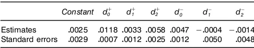
Table 8. Results of the Estimation

Standard errors 00029 00007 00012 00025 00012 00050 00048

rejected against the threshold moving average model for all statistics. The minimum of the global speciŽcation test [see Gouriéroux, Monfort, and Renault (1993)] is obtained for a threshold equal to a recession value ofƒ085. The minimum of the speciŽcation test allows judging the Žt of the model. This statistic is equal to 8.56, which has to be compared with the critical value of a chi-square with six degrees of freedom (12.59). The asymmetric moving average model is thus not rejected. The results of the estimation are given in Table 8. We see that the contemporaneous asymmetry is important, and therefore justiŽes our modeling strategy. A shock with a value greater than ƒ085 has an impact almost three times larger than a shock smaller than ƒ085. We can now exam-ine the persistence of a shock depending on its value. The persistence of shocks above and below the threshold is mea-sured by the sum of the moving average coefŽcients indexed by C and ƒ, respectively. A shock greater than the thresh-old has a persistence equal to .0209 compared to .0019 for a shock smaller than the threshold. This result corroborates the result of Beaudry and Koop (1993) obtained with an alter-native estimation strategy. Obviously, we get different results from Elwood (1998) by considering contemporaneous asym-metry and without restricting the threshold value to be zero.

6. CONCLUSION

In this article, we have analyzed how to adapt the testing procedure in indirect inference when a nuisance parameter is not identiŽed under the null hypothesis. This testing procedure has been illustrated on threshold moving average models to measure the persistence of shocks to output. A more advanced study of various TMA models and a comparison with com-peting nonlinear models such as TAR and regime-switching models is left to future research. Indeed, this requires further developments that are beyond the scope of this article, namely, the design of testing procedures for nonnested models in a dynamic setting when a nuisance parameter is involved.

ACKNOWLEDGMENTS

We beneŽted from suggestions of J. Wooldridge, an asso-ciate editor, and a referee which greatly helped us to improve the article. We thank Eric Ghysels, Éric Renault, and Jean Michel Zakoian for comments on an earlier draft. The Žrst author gratefully acknowledges Žnancial support of Fonds pour la Formation de Chercheurs et l’Aide à la recherche (FCAR). The second author gratefully acknowledges Žnancial support by the grant “Actions de Recherche Concertée” 93/98-162 from the Ministry of ScientiŽc Research (Belgian French Speaking Community). Part of this research was done when he was visiting THEMA and IRES.

APPENDIX Proof of Theorem 1

The expansions of theMestimators‚OT and‚ONT4ˆ1 ƒ5follow

from standard asymptotic arguments, and are given by

p

From the Žrst-order condition of the indirect estimator crite-rion and the above expansions [see Gouriéroux, Monfort, and Renault (1993)], we may deduce the asymptotic behavior of the indirect estimator. Indeed, as‚₀Db4ˆ₀1 ƒ5under the null for allƒ2â, we have

Hence, by Assumption 1 and the weak convergence of the score functions,

as a process indexed byƒ2â. The asymptotic distribution of W_T4¢5can be easily deduced from the asymptotic distribution ofˆON

T4¢5. The asymptotic equivalence amongWT4¢5, LMT4¢5, andLRT4¢5can be shown through modiŽcations of the proofs in Appendix 4 of Gouriéroux, Monfort, and Renault (1993) to account for the presence of the nuisance parameterƒ.

Proof of Proposition 1

The moments of the truncated standard normal variable…C t

can be calculated with the following recursive formulas:

E64…_tC57D4ƒ5 whereandêdenote the pdf and cdf of a standard Gaussian variable, respectively. Similarly, we may establish that

E64…ƒ_t 57D ƒ4ƒ5

E64…ƒ_t 527D ƒƒ4ƒ5Cê4ƒ5

E64…ƒ_t 5i_{7D ƒƒ}iƒ1_{4ƒ5C4iƒ15E64…}ƒ t5iƒ

2_{71 i¶30}

The moments of the centered processes ‡C

t D…Ct ƒE6…Ct 7

Expectations of products of powers of‡C

t and‡ƒt can sim-The conditional skewness and kurtosis of Yt can be

com-puted for any threshold ƒ by using the moments of Ut D

YtƒE6Yt—…tƒ17 and the aforementioned expressions. The

con-ditional skewness ofYt is equal to

E6U_t3—…_tƒ17

which leads to the results of Proposition 1.

Proof of Proposition 2

From the deŽnitions of the autocovariance ƒ4u5N and the centered processes‡C

Therefrom, we deduce, thanks to the iid properties of‡C t 1 ‡ƒt,

We focus on Assumptions (c), (f), (k), and (n). Other assumptions are straightforward to check.

First, we show that Sq1 T DTƒ1=2

PT

tD1sq 1t )Sq

[assump-tion (n)]. By Theorem 21.9 of Davidson (1994), uniform con-vergence overƒ2â is obtained if and only if pointwise con-vergence holds andSq1 T is stochastically equicontinuous. For

each ƒ2â, the score of instrumental models I–III takes the generic form

where u_t4ƒ5 is the error term, and the column vector x_t4ƒ5 contains lags of observed values or polynomials of these lags for the regression at time t. The pointwise multivari-ate central limit theorem then applies immedimultivari-ately to the score since Yt4ƒ5 is a q-dependent process for each ƒ. By

Andrews (1992), the existence of a Lipschitz-type condi-tion is sufŽcient to obtain stochastic equicontinuity [see also thm. 21.10 in Davidson (1994)]. We can rely here on the lines in Hansen (1996). The score is mixing at a rate inŽnitely fast sinceY_t4ƒ5isq-dependent. By establishing that the score ful-Žlls Assumption 2 in Hansen, the uniform convergence will follow. So, we have to show

˜xt4ƒ5ut4ƒ5ƒxt4ƒü5ut4ƒü5˜2µBt—ƒƒƒü—

Since the support of â is a Žnite subset of the real line, we can always Žnd a B_t<ˆ so that 2M2

t µBt—ƒƒƒü— for all ƒ1 ƒü_{2â (see Hansen (1996), p. 426). This is the desired}

result.

Now, we are interested in assumption (k). 1

T

assumptions of Lemma 1 of Hansen. Uniform almost sure con-vergence is a consequence of this lemma and the continuity of the support ofƒ.

The uniform convergence of‚ON

T4ˆ1 ƒ5[assumption (c)]

fol-lows here from assumptions (k) and (n).

Next, we have to show the uniform convergence of ï_ˆ‚ON

obvious notation. Again, by applying Lemma 1 of Hansen to 1

form almost sure convergence for these expressions. Hence, ONT4ˆ1 ƒ5 converges uniformly almost surely.

Finally, we derive the asymptotic distribution of the indirect inference estimator under the alternative. By a mean value expansion of the Žrst-order condition of the indirect estimator criterion under the alternative

pseudotrue value under the alternative. The expression above yields

Under the alternative with the appropriate selection matrixR deŽned in Section 3, we have

R0ˆüDR0ˆ0C

c p

T0

By multiplying Equation (A.1) by the selection matrixR, and by using assumptions (a)–(p), as well as results provided in the proof of Theorem 1, we obtained the desired result:

p

[Received September 1999. Revised August 2001.]

REFERENCES

Andrews, D. (1992), “Generic Uniform Convergence,”Econometric Theory, 8, 241–257.

(1993), “Tests for Parameter Instability and Structural Change With Unknown Change Point,”Econometrica, 61, 821–856.

Andrews, D., and Ploberger, W. (1994), “Optimal Tests When a Nuisance Parameter is Only Present Under the Alternative,” Econometrica, 62, 1383–1414.

Beaudry, P., and Koop, G. (1993), “Do Recessions Permanently Change Out-put?,”Journal of Monetary Economics, 31, 149–163.

Chan, K. (1990), “Testing for Threshold Autoregression,”Annals of Statistics,

18, 1886–1894.

Davidson, J. (1994),Stochastic Limit Theory: An Introduction for

Econo-metricians, Oxford, England: Oxford University Press.

Davis, R. (1977), “Hypothesis Testing When a Nuisance Parameter is Present Only Under the Alternative,”Biometrika, 64, 247–254.

(1987), “Hypothesis Testing When a Nuisance Parameter is Present Only Under the Alternative,”Biometrika, 74, 33–43.

De Gooijer, J. (1998), “On Threshold Moving-Average Models,”Journal of

Time Series Analysis, 19, 1–18.

Dhaene, G., Gouriéroux, C., and Scaillet, O. (1998), “Indirect Encompassing and Instrumental Models,”Econometrica, 66, 673–688.

DufŽe, D., and Singleton, K. J. (1993), “Simulated Moments Estimation of Markov Models of Asset Prices,”Econometrica, 61, 929–952.

El Babsiri, M., and Zako¨õan, J. M. (2001), “Contemporaneous Asymmetry in

GARCH Processes,”Journal of Econometrics, 101, 257–294.

Elwood, S. (1998), “Is the Persistence of Shocks to Output Asymmetric?,”

Journal of Monetary Economics, 41, 411–426.

Gallant, R., and Tauchen, G. (1996), “Which Moments to Match?,”

Econo-metric Theory, 12, 657–681.

Ghysels, E., Guay, A., and Hall, A. (1998), “Predictive Tests for Struc-tural Change With Unknown Breakpoint,”Journal of Econometrics, 82, 209–233.

Ghysels, E., and Guay, A. (2001a), “Structural Change Tests for Simulated Method of Moments,”Journal of Econometrics, (forthcoming).

(2001b), “Indirect Inference, EfŽcient Method of Moments and Struc-tural Change,” mimeo.

Gouriéroux, C., and Monfort, A. (1995a), Simulation Based Econometric

Methods, CORE Lecture Series and Oxford University Press.

(1995b), “Testing, Encompassing and Simulating Dynamic Econo-metric Models,”Econometric Theory, 11, 195–228.

Gouriéroux, C., Monfort, A., and Renault, E. (1993), “Indirect Inference,”

Journal of Applied Econometrics, 8, 85–118.

Hansen, B. (1996), “Inference When a Nuisance Parameter is not IdentiŽed Under the Null Hypothesis,”Econometrica, 64, 413–430.

Michaelides, A., and Ng, S. (2000), “Estimating the Rational Expec-tations Model of Speculative Storage: A Monte Carlo Compari-son of Three Simulation Estimators,” Journal of Econometrics, 96,

231–266.

Pollard, D. (1994),Convergence of Stochastic Processes, New York: Springer-Verlag.

Smith, A. (1993), “Estimating Nonlinear Time-Series Models Using Sim-ulated Vector Autoregressions,” Journal of Applied Econometrics, 8,

63–84.

Sowell, F. (1996), “Optimal Tests for Parameter Instability in the Generalized Method of Moments Framework,”Econometrica, 64, 1085–1107. Tong, H. (1990),Non-Linear Time Series: A Dynamical Systems Approach,

Berlin: Springer.

Wecker, W. (1981), “Asymmetric Time Series,”Journal of the American Sta-tistical Association, 76, 16–21.

Zako¨õan, J.-M. (1994), “Threshold Heteroskedastic Models,”Journal of

Eco-nomic Dynamics and Control, 18, 931–955.