Full Terms & Conditions of access and use can be found at
http://www.tandfonline.com/action/journalInformation?journalCode=ubes20
Download by: [Universitas Maritim Raja Ali Haji] Date: 13 January 2016, At: 00:19
Journal of Business & Economic Statistics
ISSN: 0735-0015 (Print) 1537-2707 (Online) Journal homepage: http://www.tandfonline.com/loi/ubes20
Bayesian Analysis of the Heterogeneity Model
Sylvia Frühwirth-Schnatter, Regina Tüchler & Thomas Otter
To cite this article: Sylvia Frühwirth-Schnatter, Regina Tüchler & Thomas Otter (2004) Bayesian Analysis of the Heterogeneity Model, Journal of Business & Economic Statistics, 22:1, 2-15, DOI: 10.1198/073500103288619331
To link to this article: http://dx.doi.org/10.1198/073500103288619331
Published online: 01 Jan 2012.
Submit your article to this journal
Article views: 67
View related articles
Bayesian Analysis of the Heterogeneity Model
Sylvia FRÜHWIRTH-SCHNATTER
Department of Applied Statistics (IFAS), Johannes Kepler Universität, A-4040 Linz, Austria
(Sylvia.Fruehwirth-Schnatter@jku.at)
Regina T
ÜCHLERDepartment of Statistics, University of Business Administration and Economics, A-1090 Vienna, Austria
(regina.tuechler@wu.edu)
Thomas OTTER
Fisher College of Business, Ohio State University, 2100 Neil Avenue, Columbus, OH 43210
(otter–2@cob.osu.edu)
We consider Bayesian estimation of a nite mixture of models with random effects, which is also known as the heterogeneity model. First, we discuss the properties of various Markov chain Monte Carlo sam-plers that are obtained from full conditional Gibbs sampling by grouping and collapsing. Whereas full conditional Gibbs sampling turns out to be sensitive to the parameterization chosen for the mean struc-ture of the model, the alternative sampler is robust in this respect. However, the logical extension of the approach to the sampling of the group variances does not further increase the efciency of the sampler. Second, we deal with the identiability problem due to the arbitrary labeling within the model. Finally, a case study involving metric conjoint analysis serves as a practical illustration.
KEY WORDS: Collapsing; Conjoint analysis; Grouping; Label switching; Mixture of random-effects model; Parameterization.
1. INTRODUCTION
In this article we consider the heterogeneity model
yiDX1i®CX
2
i¯iC"i; "i»N.0; ¾"2I/; iD1; : : : ;N;
(1) whereyi is a vector ofTiobservations for subjecti,X1i is the Ti£dmatrix for thed£1 vector of the xed effects®, andX2i is the design matrix of dimensionTi£rfor ther£1 random-effects vector¯i. I is the identity matrix.¯i is a random ef-fect that, due to unobserved heterogeneity, is different for each subject. The unknown distribution¼.¯i/of heterogeneity is ap-proximated by a mixture distribution,
¯i»
K
X
kD1
´kN.¯Gk;QGk/; (2)
with the unknown group means ¯G1; : : : ;¯GK, the unknown group covariance matrices QG1; : : : ;QGK, and the unknown group probabilities ´ D.´1; : : : ; ´K/. Model (1) is a nite mixture of models with random effects. This model, but with
QG1; : : : ;QGK being the same in all groups, was introduced by Verbeke and Lesaffre (1996). Later, Verbeke and Molenberghs (2000) introduced the terminology heterogeneity model for (1). A comparable model without xed effects has been studied by Allenby, Arora, and Ginter (1998) for logit choice models and by Lenk and DeSarbo (2000) for observations from distribu-tions of general exponential families. In this article, however, we conne ourselves to the important special case of observa-tions from the normal distribution.
Bayesian estimation of the heterogeneity model has been dis-cussed by Allenby et al. (1998) and Lenk and DeSarbo (2000). Bayesian estimation starts by introducing discrete latent group indicatorsSi;iD1; : : : ;N, taking values inf1; : : : ;Kgwith un-known probability distribution Pr.SiDk/D´k,kD1; : : : ;K.
With the help of the latent group indicators, model (2) is writ-ten as
¯i»
8 > < > :
N.¯G1;QG1/ ifSiD1
:: :
N.¯GK;QGK/ ifSiDK.
(3)
All unknown quantities, including the latent random effects
¯N D.¯1; : : : ;¯N/, the latent indicators SN D.S1; : : : ;SN/ and the unknown model parametersÁD.ÁL;ÁV;´/, are es-timated jointly using Markov chain Monte Carlo (MCMC) simulation from their posterior density. We use the notation
ÁL D.®;¯G1; : : : ;¯GK/ for the location parameters andÁV D
.QG1; : : : ;QGK; ¾"2/ for the variance parameters. A straightfor-ward MCMC method is to split the augmented parameter into blocks and sample the variables in each block from their full conditionals.
Algorithm 1(Sampling from full conditionals). (i-1) SampleSNfrom¼.SNj¯N;Á;yN/. (ii-1) Sample´from¼.´jSN/.
(iii-1a) Sample®from¼.®j¯N;SN;¯G1; : : : ;¯GK;ÁV;yN/. (iii-1b) Sample¯G1; : : : ;¯GK from¼.¯G1; : : : ;¯GKj¯N;SN;®;
ÁV;yN/.
(iii-1c) Sample¯N from¼.¯NjSN;Á;yN/. (iv-1) SampleÁVfrom¼.ÁVj¯N;SN;ÁL;yN/.
A comparable full conditional Gibbs sampler, but with step (ii-1) replaced by
(ii-1) Sample ´ from ¼.´jSN/ under the restriction ´1 <
¢ ¢ ¢< ´K (constrained Algorithm 1),
© 2004 American Statistical Association Journal of Business & Economic Statistics January 2004, Vol. 22, No. 1 DOI 10.1198/073500103288619331
2
has been applied successfully in marketing science in the pio-neering work of Allenby et al. (1998) and Lenk and DeSarbo (2000). Although Algorithm 1 happened to work ne in these applications, it is necessary to discuss potential pitfalls of this algorithm and to consider alternative methods of MCMC esti-mation of model (1).
A rst potential drawback of Algorithm 1—either con-strained or unconcon-strained—is that in case that correlations are high between quantities in the different subblocks, especially within step (iii), the resulting sampler will be slowly mixing. This is a well-discussed issue for the normal linear mixed model (Gelfand, Sahu, and Carlin 1995) which is a special case of the heterogeneity model withKD1. We demonstrate in this article that similar problems are to be expected for the general model where K>1 and the case study in Section 4.3 highlights the rather dramatic consequences for practical work. Algorithm 1 turns out to be sensitive to the parameterization used for the mean structure of model (1) and might exhibit slow conver-gence in cases where random effects with low variance are centered around the group means and in cases where random effects with high variance are centered around0.
As an alternative to Algorithm 1, we exploit a common way of overcoming mixing problems caused by correlation, namely “blocking” (i.e., updating parameters jointly) and “collapsing” (i.e., sampling parameters from partially marginalized distribu-tions) (see Chen, Shao, and Ibrahim 2000; Liu, Wong, and Kong 1994). Such blocked and collapsed samplers have been derived for a normal linear mixed model independently by Chib and Carlin (1999) and Frühwirth-Schnatter and Otter (1999); in this article, we extend them to the mixture of random-effects mod-els (1) withK>1. To our knowledge, such a collapsed sam-pler has not yet been considered for the general heterogeneity model. This alternative sampler will turn out to be robust to the parameterization underlying the mean structure. The resulting sampler is only partly marginalized; in the sense that all vari-ance parameters are still sampled from their full conditionaldis-tributions. Marginalizingthis part of the sampling scheme is not possible without leaving the convenient Gibbs sampling frame-work. However, by introducing a Metropolis–Hastings step into the sampler, we are able to investigate the merits of “collaps-ing” this sampling step. Interestingly, this fully marginalized MCMC scheme (in the sense that no sampling step conditions on the random effects) does not provide a noticeable improve-ment over the partly marginalized sampler.
The second topic of this article concerns the identiability problem inherent in model (1). Because model (1) includes the latent, discrete structure SN, the unconstrained posterior typically is multimodal. The impact of this type of unidenti-ability on MCMC estimation of mixture models has been dis-cussed by Stephens (2000), Celeux, Hurn, and Robert (2000), and Frühwirth-Schnatter (2001a). In this article we add some more aspects on this identiability problem and illustrate for simulated data that a standard constraint as the one applied in step (ii-1) of the constrained Algorithm 1 does not neces-sarily restrict the posterior simulations to a unique modal re-gion. Choosing of a suitable identiability constraint appears particularly difcult in the multivariate setting considered here. We will demonstrate within a case study from metric conjoint analysis how to explore MCMC simulations from the
uncon-strained posterior to obtain an identiability constraint that is able to separate the posterior modes.
The rest of the article is organized as follows. In Section 2 we discuss, starting from Algorithm 1, various MCMC sam-plers obtained from Algorithm 1 by grouping and collapsing. In Section 3 we explore the unidentiability problem. We present an empirical illustration involving metric conjoint analysis in Section 4, and conclude the article with some nal remarks in Section 5.
2. PARAMETERIZATION, GROUPING, AND COLLAPSING
2.1 Parameterization and Sampling From the Full Conditionals
A straightforward method for MCMC estimation of the gen-eral heterogeneity model (1) is sampling from the full condi-tionals (Algorithm 1 in Sec. 1). The problem with sampling from the full conditionals is that in cases where correlations are high between quantities in different subblocks, the resulting sampler will be slowly mixing. The possible inuence of the parameterization on the efciency of the MCMC sampler, espe-cially within step (iii-1), is a well-discussed issue for the normal linear mixed model (Gelfand et al. 1995). Because this model is the special case of (1) whereKD1, we expect a similar inu-ence of the parameterization for the more general model, which, conditional onSN, could be regarded as the combination ofK normal linear mixed models with the random effects of each group independent from each other.
2.1.1 Centered and Noncentered Parameterization. The mean structure of model (1) can be parameterized in two com-mon ways. If X1i and X2i do not have any common column, then ® represents parameters that are xed for all individu-als, whereas ¯i are the random (heterogeneous) effects cen-tered around¯Gk, the population mean in classk:E.¯ijSiDk;
Á/D¯Gk. The expectation of the marginal distribution of yi, where both the random effects and the latent indicators are in-tegrated out, is given by
E.yijÁ/DX1i®CX2i®¯; ®¯D K
X
kD1
¯Gk´k: (4)
ConditionalonSi, centering is around the group-specic means, whereas marginally (where the indicators are integrated out), the random effects are centered around the population mean, E.¯ijÁ/D®¯. Therefore, this parameterization seems to be rather close to the idea of hierarchical centering introduced by Gelfand et al. (1995), and thus we call itcentered parameteriza-tion. This is the parameterization used by Allenby et al. (1998) and Lenk and DeSarbo (2000).
Alternatively, Verbeke and Lesaffre (1996) designed mo-del (1) in such a way that X1i and X2i may have common columns. This implies the additional constraint that marginally (where the indicators are integrated out) the random effects are deviations from the xed effects with mean0,E.¯ijÁ/D
PK kD1¯
G
k´k D0. The rst two moments of the marginal dis-tribution ofyi, where both the random effects and the latent
indicators are integrated out, are given by
Like in the classical random-effects model, the random effects contribute to the variance of yi only. Because marginally, the random effects are centered around0, we term this parameteri-zationnoncentered(as in Gelfand et al. 1995).
The two parameterizations are, of course, related. Given the centered parameterization, the noncentered parameterization is obtained by adding®¯ to the xed effects, where®¯ is dened in (4) as the weighted mean of the group-specic parameters, and by subtracting®¯ from each¯i,
Although the two parameterizations are theoretically equiva-lent, the choice of the parameterization might have a substantial inuence on the efciency of a MCMC sampler.
We discuss this in more detail for a model without xed ef-fects (X1i D0 in the centered parameterization and X1i DX2i
in the noncentered parameterization). In the context of a single normal linear mixed model (i.e.,KD1), Gelfand et al. (1995) recommended selecting the parameterization according to the contribution of the random-effects covariance matrix QG to the marginal variance ofyi. The noncentered parameterization should be used only if the contribution of the random effects to the marginal variance is small compared with the contribution of the observation error ¾"2. If the variance of the random ef-fects is dominating the variance of the marginal model, then the centered parameterization should be used.
These results are easily extended to the mixture of random-effects models considered here. Conditional onSN, model (1) may be regarded as a single random-effects model with hetero-geneous covariance matrix QiDQGS
i. The results of Gelfand et al. (1995, sec. 2), are easily extended to such a model. The crucial quantity is the determinant of the matrix
QiB¡i 1DQi
¡
¾"¡2.X2i/0X2i CQi¡1¢D¾"¡2Qi.X2i/0X
2
i CI; (7) which reects the contribution of the random effects to the marginal variance ofyi. We obtain the following results. The centered parameterization is to be preferred if jBiQ¡i 1j D 1=jQiB¡i 1jis near 0, whereas the noncentered parameterization is to be preferred ifjBiQ¡i 1j D1=jQiB¡i 1jis close to 1.
These results suggest using the parameterization of Verbeke and Lesaffre (1996) in the context whereK>1 only in cases where the variability of the random effects is small compared to the observation error¾"2 forall groupsand to use the cen-tered parameterization as was done by, for example, Lenk and DeSarbo (2000) in those cases where forall groupsthe variabil-ity of the random effects is large compared to the observation error¾"2. Both parameterizations may be poor if for one group all effects are nearly homogeneous, whereas for the other group heterogeneity dominates. Our experiences with simulated data (reported in the next section), as well as with real data, conrm these ndings.
2.1.2 Illustrative Example. Consider a simplistic metric conjoint study with a controlled full-factorial design, where Nconsumers evaluate two attributes of a product, one being, for instance, one of two brands, and the second being some metric attribute that is either low or high,
yiDX2i¯iC"i; X2i D
whereyiis the purchase likelihood on a given scale. We assume that there are two groups of consumers with heterogeneityin the preferences,
Whether we should combine full conditional Gibbs sampling with the parameterization of Lenk and DeSarbo (2000) or rewrite the model following Lesaffre and Verbeke (1996) de-pends on the amount of unobserved heterogeneity. In our ex-ample,
² Use the noncentered parameterization if for all groups heterogeneity is small for all effects compared with
¾"2.±11; ±12; ±13; ±21; ±22; ±23¿¾"2/.
² Use the centered parameterization if for each group at least oneeffect dominates the marginal variance ofyi. This result also holds if one of the other effects is nearly homo-geneous (e.g.,±k3¿¾"2, whereas±k2À¾"2).
To illustrate these results, we simulated data and compared the output from Algorithm 1 for the two different parameteriza-tions. The MCMC samples are compared by the lag 1 sample autocorrelation of the MCMC chain as well as by the inef-ciency factor·, which accounts for the whole serial dependence in the sampled values (Geweke 1992),
·D1C2
where½ .j/represents the autocorrelation at lagjof the sampled parameter values.·is the factor by which we have to increase the run length of the MCMC sampler compared to iid sampling. We choose the bandwidthJ such that½.J/ signicantly con-tributes to the serial dependence of the sampled value but the succeeding½ .j/,jDJC1;JC2; : : : ;are not signicant. These are contained in the interval½ .j/2[¡2=pM;2=pM], where Mis the number of MCMC draws.
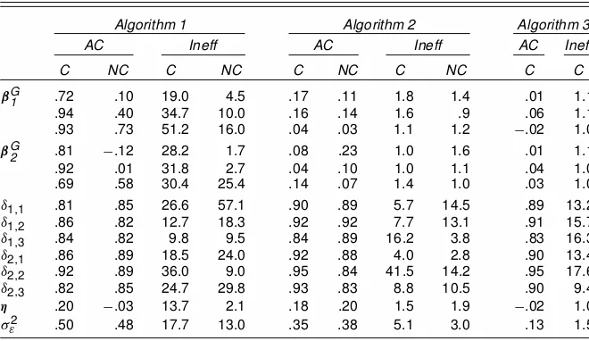
Table 1. Simulation 1, Autocorrelation at Lag 1 (AC) and Inefciency Factors (Ineff) for the Three Sample Algorithms (Algorithms 1–3) and the Centered (C) and
the Noncentered (NC) Parameterization
Algorithm 1 Algorithm 2 Algorithm 3
AC Ineff AC Ineff AC Ineff
C NC C NC C NC C NC C C
¯G1 .72 .10 19.0 4.5 .17 .11 1.8 1.4 .01 1.1
.94 .40 34.7 10.0 .16 .14 1.6 .9 .06 1.1 .93 .73 51.2 16.0 .04 .03 1.1 1.2 ¡.02 1.0
¯G2 .81 ¡.12 28.2 1.7 .08 .23 1.0 1.6 .01 1.1
.92 .01 31.8 2.7 .04 .10 1.0 1.1 .04 1.0 .69 .58 30.4 25.4 .14 .07 1.4 1.0 .03 1.0
±1;1 .81 .85 26.6 57.1 .90 .89 5.7 14.5 .89 13.2
±1;2 .86 .82 12.7 18.3 .92 .92 7.7 13.1 .91 15.7
±1;3 .84 .82 9.8 9.5 .84 .89 16.2 3.8 .83 16.3
±2;1 .86 .89 18.5 24.0 .92 .88 4.0 2.8 .90 13.4
±2;2 .92 .89 36.0 9.0 .95 .84 41.5 14.2 .95 17.6
±2;3 .82 .85 24.7 29.8 .93 .83 8.8 10.5 .90 9.4
´ .20 ¡.03 13.7 2.1 .18 .20 1.5 1.9 ¡.02 1.0
¾"2 .50 .48 17.7 13.0 .35 .38 5.1 3.0 .13 1.5
Simulation 1. The data for the rst simulation come from (8) with the group specic means ¯G1 D.15 3 ¡:8/0 and ¯G2 D
.7 7¡2/0. We takeQG1 Ddiag.1 1:5/andQG2 Ddiag.1:5 1:5 1/
for the group variances and¾"2D10 for the observation error variance. The group weights are ´1D:6 and´2D:4. We
sim-ulate 200 vectors,yi, and run Algorithm 1 for each of the two parameterizations for 1,500 iterations. The last 1,000 iterations are kept for estimation. The simulations are based on a nor-mal prior for the group-specic means,¯Gk »N..11 5¡1:4/0;
10¢I/,kD1;2; an inverted Wishart prior for the group-specic covariance matrices, QGk » IW.5;diag.3:75 3:75 3:25//, kD1;2; and a Dirichlet prior for the group weights,´»D.1;1/. We remain noninformative about the model error variance¾"2. From (7) and (10), we obtain E.jBiQ¡i 1j/D:9198, support-ing theoretically the noncentered parameterization. This is con-rmed empirically. It is obvious from the autocorrelations and the inefciency factors of the group-specic means in Table 1 that the noncentered parameterization is more efcient than the
centered parameterization. Loss of efciency due to the cen-tered parameterization is prominent when sampling the group-specic means¯Gk and´.
Simulation 2. In this simulation we simulate data for the case where for each group the variance for at least one effect dom-inates the observation equations variance. We have the same group means and group weights as in simulation 1, but now takeQG1 Ddiag.10 10:5/,QG2 Ddiag.1:5 1:5 6/, and¾"2D1. Again we simulate 200 vectors,yi, and run Algorithm 1 for each of the two parameterizations for 1,500 iterations, with the nal 1,000 iterations kept for estimation. We use the same prior information as for simulation 1, only the prior for the groups covariances is changed toQGk »IW.5;diag.18 18 9//,kD1;2. From (7) and (10), we obtain E.jBiQ¡i 1j/D:0012, support-ing theoretically the centered parameterization. The autocorre-lations and the inefciency factors in Table 2 clearly indicate that the centered parameterization works better.
Table 2. Simulation 2, Autocorrelation at Lag 1 (AC) and Inefciency Factors (Ineff) for the Three Sample Algorithms (Algorithms 1–3) and the Centered (C) and
the Noncentered (NC) Parameterization
Algorithm 1 Algorithm 2 Algorithm 3
AC Ineff AC Ineff AC Ineff
C NC C NC C NC C NC C C
¯G1 .24 .25 2.3 17.0 .15 .24 1.2 4.0 .05 1.1
.05 .52 1.0 17.7 .04 .04 1.4 1.0 .05 1.1 .05 .40 1.1 5.1 .04 ¡.03 1.0 1.0 ¡.07 1.0
¯G2 .06 .19 3.3 4.7 .09 .05 1.1 2.3 .10 1.2
.07 .25 2.0 4.5 .04 .01 1.0 1.0 .00 1.0
¡.01 .81 1.7 34.2 ¡.02 .01 1.0 1.0 .02 1.0
±1;1 .27 .30 1.0 2.1 .33 .41 1.0 3.4 .51 2.3
±1;2 .21 .17 1.0 1.1 .20 .28 1.0 1.0 .47 3.0
±1;3 .51 .53 2.3 1.0 .46 .55 2.0 1.0 .71 2.9
±2;1 .47 .54 1.8 2.7 .52 .50 1.0 4.3 .50 2.3
±2;2 .51 .50 1.0 1.4 .49 .46 1.1 2.8 .49 1.5
±2;3 .25 .26 1.0 1.0 .36 .22 1.0 1.0 .22 1.5
´ .11 .09 1.0 5.9 .10 .18 1.0 2.2 .03 1.1
¾2
" .37 .72 5.0 1.6 .70 .70 4.4 5.9 .07 1.2
2.2 Sampling From Partially Marginalized Conditionals
We demonstrated in the last section that choosing the wrong parameterization may cause slow convergence for a sampler that is based on sampling xed effects ® and the heteroge-neous effects¯N from the full conditionals. Rather than trying to nd the right parameterization for the case study at hand, one could apply a sampler that is insensitive to the parameterization. Note that a suitable parameterization does not exist for the case ofK>1, where at least one group is close to homogeneity and at least one other group is characterized by random-effects vari-ances that dominate the observation error variance.
Common methods of constructing such a sampler are block-ing, such that parameters are sampled jointly, and collapsblock-ing, where full conditional densities are substituted by marginal densities. The latter are obtained from integrating out part of the conditioning parameters.
The experiences reported for a normal linear mixed model by Chib and Carlin (1999) and Frühwirth-Schnatter and Otter (1999) suggest that it is desirable to group the xed effects and the group-specic means and to sample them from the density where the random effects are integrated out. Furthermore, from the result reported by Gerlach, Carter, and Kohn (2000), we expect that it is also desirable to sample the group indicators from the density where the random effects are integrated out. This leads to the following sampler:
Algorithm 2 (Sampling from partially marginalized condi-tionals).
(i-2) SampleSN from¼.SNjÁ;yN/. (ii-2) Sample´from¼.´jSN/.
(iii-2) Sample ÁL, the xed effects and the group-specic means, and ¯N, the random effects, conditional on
SN;ÁV, and yN from the joint normal distribution
Note that only steps (i) and (iii) differ between Algorithms 1 and 2. In step (i-2), we use a collapsed sampler for SN, where instead of sampling from the full conditional density
¼.SNj¯N;Á;yN/, we sample from the marginal conditional density ¼.SNjÁ;yN/, where the random effects ¯N are in-tegrated out. In step (iii-2) we use a blocked sampler for jointly sampling ®;¯G1; : : : ;¯GK;¯N rather than sampling ®,
.¯G1; : : : ;¯GK/, and¯N in three different blocks conditional on the other parameters. Step (iii-2a) amounts to sampling the lo-cation parametersÁLD.®;¯G1; : : : ; ¯GK/from the conditional density¼.ÁLjSN;ÁV;yN/, where again the random effects¯N
are integrated out.
To sample from the marginal conditional posterior densities in Algorithm 2, we derive the marginal model from (1), where the random effects are integrated out. Conditional on SN, the mixture of random-effects model (1) is a single mixed-effects model with heterogeneity in the variance of the random effects:
yiDX1i®CX More details on steps (i-2), (iii-2), and (iv-2) are given in Appendix B. The following example demonstrates that this marginalization leads to a sampler that is insensitive to the se-lected parameterization of the mean structure.
Simulations 1 and 2(Continued). We are now going to ap-ply Algorithm 2 to Simulation 1 and 2 from the previous sec-tion.
From Algorithm 2’s lag 1 sample autocorrelations and the inefciency factors in Tables 1 and 2, we cannot make out any difference between the two methods of parameterization when sampling¯Gk. Thus Algorithm 2 actually proves insensitive to the parameterization chosen for the mean structure. When we compare the values for¯Gk sampled by Algorithm 2 with the ones derived by Algorithm 1, we see that the partial marginal-ization leads to lower autocorrelations, as well as to improved efciency.
2.3 Sampling From the Marginal Model
One special feature of Algorithm 2 is that the parametersÁL
appearing in the mean structure, as well as the group indi-cators SN, are sampled from the marginal model, where the random effects are integrated out, whereas the variance para-metersÁV are sampled from the full conditional model. The reason for this is that despite marginalization over the random effects, the conditional densities of the mean parameters ÁL
are from a well-known distribution family (multivariate nor-mal), whereas the marginal distribution of the variance para-meters ¼.ÁVjÁL;SN;yN/ where the random effects are inte-grated out does not belong to a well-known family. However, the functional value of the nonnormalized marginal density
¼?.ÁVjÁL;SN;yN/is available from
From the marginal model (13), we obtain that the likelihood L.yij®;¯Gk;QGk; ¾
2
"/is the likelihood of the normal distribution
N.yiIX1i®CX2i¯Gk;X2iQGk.X2i/0C¾"2I/.
Because the nonnormalized density ¼?.ÁVjÁL;SN;yN/ is available in closed form, we use the Metropolis–Hastings algo-rithm to sampleÁV from¼.ÁVjÁL;SN;yN/. Details are given in Appendix C, where we use a mixture of inverted Wishart densities as a proposal density.
Algorithm 3(Sampling from fully marginalized condition-als).
(i-3) SampleSN from¼.SNjÁ;yN/. (ii-3) Sample´from¼.´jSN/.
(iii-3) Sample all xed effects, random effects, and group-specic means ÁL;¯N conditional on SN, ÁV, yN
from the joint normal distribution ¼.ÁL;¯NjSN;
ÁV;yN/, as in (iii-2).
(iv-3) Sample the variance parametersÁVconditionalonÁL,
SN,yN, where the random effects are integrated out: (iv-3a) For kD1; : : : ;K, sample QGk from ¼.QGkj
QG¡k; ¾"2;ÁL;SN;yN/, whereQG¡kdenotes all covariance matrices butQGk.
(iv-3b) Sample ¾"2 from ¼.¾"2jQG1; : : : ;QGK;ÁL;
SN;yN/.
Simulations 1 and 2 (Continued). We applied Algorithm 3 to our simulated data. Because of the invariance to the parame-terization (see Sec. 2.2), we use only the centered parameteri-zation here. To compare the performance of this algorithm with the performance of Algorithms 1 and 2, we listed the autocorre-lations at lag 1 and the inefciency factors in Tables 1 and 2. We carry out 3,000 iterations and keep the last 2,000 for estimation. We see that the Metropolis–Hastings step did not lead to bet-ter behavior of the sampler for the group-specic variances for either Simulation 1 or Simulation 2. Only the model error vari-ance¾"2 may be sampled more efciently by the Metropolis– Hastings step.
3. DEALING WITH UNIDENTIFIABILITY
3.1 About Unidentiability and Label Switching
In what follows we use the notationà D.¯N;SN;Á/to de-note all unknown parameters andAto denote the unconstrained parameter space. The unconstrained parameter space A con-sists of K! disjunct subspacesL 1; : : : ;L K!, differing only in the way of labeling the groups,ADSK!
lD1L l. To each labeling
subspaceL lcorresponds a certain permutation½loff1; : : : ;Kg telling us with which of theKgroups the various group-specic components of a parameterÃ2Ahave to be associated. With-out loss of generality, we may assume that½1.¢/is equal to the
identity. Therefore, ifÃ2L 1, then for eachkD1; : : : ;K, the components.¯Gk;QGk; ´k/ ofÁ correspond to group k. In L l with l>1, however,.¯Gk;QGk; ´k/correspond to group½l.k/ rather thank as before. This label switching between the la-beling subspaces causes the unconstrained posterior to have multiple, at most K!, modes. The modes are equivalent if the prior¼.Á/is invariant to relabeling the groups.
For Bayesian estimation via MCMC methods, it is essen-tial to produce draws from a unique labeling subspace, if inter-est lies in inter-estimation of group-specic parameters such as¯Gk,
QGk,´k or classication probabilities Pr.SiDkjyN/. Otherwise, label switching could be present, rendering meaningless any es-timation of group-specic parameters from the MCMC output. There is a geometric aspect to the identication of a unique la-beling in that simulations are conned to onlyoneof the K! possible modal regions.
It is important to emphasize that identifying a unique label-ing is different from formal identiability achieved by intro-ducing a constraint,R. In general, an identiability constraint is dened in terms of a subset Rof the unrestricted parame-ter spaceA, such that for all parametersÃ2A,½ .Ã/2Rfor exactly one permutation½Ã.¢/(see Stephens 1997, p. 43). An example would be the following constraint on the weights:
R´:´1<¢ ¢ ¢< ´K; (16)
which was applied by Aitkin and Rubin (1985) and Lenk and DeSarbo (2000) as a standard constraint for this type of mixture models. But this constraint may be an order relation for a sin-gle component of the group-specic parameter or may involve more than one component. With an identiability constraintR, formal identiability is achieved in the sense that if two para-metersÁandÁQ dene the same probability law for all possible observationsyN, thenÁandÁQ need to be the same:
L.yNjÁ/DL.yNj QÁ/ ¡! ÁD QÁ: (17) L.yNjÁ/is the marginal likelihood, where .¯N;SN/are inte-grated out.
It is a common misunderstanding that formal identiabil-ity through anarbitraryidentiability constraintRleads to a unique labeling. This is not necessarily the case. An identia-bility constraint restricts the parameter spaceAto a subspace in which no two different parameters dene the same probability law to achieve (17). But the parameters in this subspace need not come from one labeling subspace—or, in more geometric terms, from one modal region. As a consequence, if Bayesian analysis is carried out on that subspace dened by the identia-bility constraintR, then label switching might still be present. An identiability constraint will lead to a unique labeling only if it respects the geometry of the posterior and is able to separate the modes of the unconstrained posterior.
For illustration, we simulated 200 datasets, each containing ND100 bivariate observations from the four-component mix-ture model
yt»´1N.ytI¹1;6/C´2N.ytI¹2;6/
C´3N.ytI¹3;6/C´4N.ytI¹4;6/; (18)
where ´D.:1 :24 :26 :4/0, ¹1D.¡2 ¡2/0, ¹2D.¡2 2/0,
¹3D.2¡2/0,¹4D.2 2/0, and6D¾2¢Iwith¾2D:01 and the identity matrixI. This is a simple special case of model (1) withQG1 D ¢ ¢ ¢ DQGKD0,X1i D0,X2i DI, and¯Gk D¹k.
To illustrate the difference between the unconstrained and the constrained posterior, Figure 1 shows simulations from vari-ous bivariate marginal densities,¼.¹k;1; ¹k;2jyN/,kD1; : : : ;4,
for one randomly selected dataset. All simulations are based on the prior distributions¹j»N.0;4¢I/,¾2»IG.2; :01/and
´»D.4; : : : ;4/ and were obtained by permutation sampling (see Frühwirth-Schnatter 2001a). The rst row shows simula-tions from the unconstrained posterior, which obviously has multiple modes and is invariant to permutationsof the labels (all four gures are identical). The second row shows simulations from the constrained posterior under the constraint (16) on the weights,R´:´1<¢ ¢ ¢< ´4. Obviously the simulations exhibit
label switching. Because two of the groups have weights that, although different, are close to each other, we achieve formal identication by constraint (16) but no unique labeling. From the simulations shown in the rst row of Figure 1, a constraint that separates the four modal regions can be easily found. One possibility is the following constraint on the means:
R2: max.¹1;1; ¹2;1/ <min.¹3;1; ¹4;1/;
¹1;2< ¹2;2; ¹3;2< ¹4;2: (19)
To emphasize the difference between formal identication within a likelihood analysis and unique labeling within a
Figure 1. Simulations From the Various Bivariate Marginal Densities¼.¹k;1; ¹k;2jyN/for KD4. First row, random permutation sampling from the unconstrained posterior; second row, permutation sampling under constraint (16); last row, permutation sampling under constraint (19).
Bayesian analysis, the last row in Figure 1 shows simulations from the various bivariate marginal densities¼.¹k;1; ¹k;2jyN/
under constraint (19). In contrast with constraint (16), this con-straint induces a unique labeling.
The fact that formal identication by constraint (16) does not necessarily induce a unique labeling remains undetected if a MCMC sampler is used for constrained estimation that sticks at the current labeling subspace. An example is the slice sampler discussed by Lenk and DeSarbo (2000). As can be seen from comparing the rst and second rows of Figure 2, the draws from slice sampling under constraint (16) stay within one labeling
Figure 2. Simulations From the Various Bivariate Marginal Densities
¼.¹3;1; ¹3;2jyN/,¼ .¹3;1; ´3jyN/and¼ .¹3;2; ´3jyN/for KD4. First row, permutation sampling under constraint (16); second row, slice sam-pling under constraint (16).
subspace only, missing part of the parameter space constrained toR´. This might introduce a bias toward the constraint in com-parison to draws obtained under constraint (19), which induces a unique labeling.
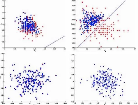
The inuence of the constraint is evident from Figure 3, in which we compare the posterior estimates of´and¹obtained from permutation sampling under constraint (19) with slice sampling under constraint (16) for all 200 simulated datasets. Whereas a bias toward the constraint´2< ´3 is introduced
for´2and´3, the constraint causes less variation of´1and´4
around the true values, and has no effect on estimation of¹. Whether or not this bias matters depends on what inference we draw from the simulations. (See Frühwirth-Schnatter 1999 for discussion on the considerable effect of this bias on esti-mates of the model likelihood.) Assume in the present context that we want to estimate the differenceDbetween various group sizes,
DD
Á´
2¡´1
´3¡´2
´4¡´3
!
; (20)
with the true value beingDD.:14; :02; :14/. If we want to ob-tain an estimator with small systematic error (i.e., small bias
O
D¡D), then the bias introduced by constraintR´ of course matters (Table 3). If we are interested in obtaining an
(possi-Table 3. Comparing Slice Sampling Under Constraint (16) and Permutation Sampling Under Constraint (16)
´2¡´1 ´3¡´2 ´4¡´3
Bias Slice sampling ¡.0394 .0368 ¡.0229 Permutation ¡.0182 ¡.00555 ¡.0159
sampling
Mean Slice sampling .00261 .00190 .00285 squared error Permutation .00314 .00394 .00479
sampling
Figure 3. Posterior Estimates Obtained for 200 Datasets Simulated From Model (18)., permutation sampling under constraint (19);², slice sampling under constraint (16);C, true value.
bly biased) estimator with small variance around the true value [i.e., small mean squared error.DO¡D/2], then the bias does not matter as long as it is small compared with the variation of the estimator. For the present case study, the biased estimator has even smaller mean squared error than the estimator obtained from constraint (19) (see Table 3).
3.2 Statistical Inference From the Unidentied Model
We emphasize that for many estimation problems arising in the empirical analysis of the mixtures of random effects models, identifying a unique labeling is not necessary. This is the case if we want to estimate a functional of the augmented parameter vectorf.Ã/that is invariant to relabeling the indices. For such a functional, the expectation with respect to posterior simulations constrained to any of the unique labeling subspaces is equal to the expectation with respect to posterior simulations from the unconstrained spaceA,
ELl
¡
f.Ã/jyN¢DELs
¡
f.Ã/jyN¢DEA
¡
f.Ã/jyN¢: (21)
A proof of (21) is given in Appendix D. A practical conse-quence of (21) is that many quantities may be estimated without introducing a unique labeling. Among these quantities are ob-viously parameters that are common to all components of the
mixture, such as® and¾"2, and, notably, theindividual para-meters¯i, because
¯i»
K
X
kD1
´kN.¯Gk;Q G k/D
K
X
kD1
´½.k/N
¡
¯G½.k/;QG½.k/¢:
Consequently, the behavior of each subject under designsX1;?i ,
X2;?i different from that used for estimation may be predicted without a unique labeling. Further example for quantities that are invariant to relabeling are all moments of the distribution of heterogeneity, for example, the mean or the covariance matrix
®¯D
K
X
kD1
¯Gk´k; QD K
X
kD1
¡
¯Gk.¯Gk/0CQGk¢´k¡®¯®¯0:
4. AN EMPIRICAL STUDY FROM METRIC CONJOINT ANALYSIS
4.1 The Data and the Model
The data come from a brand–price trade-off study in the min-eral water category. Each of 213 Austrian consumers stated their likelihood of purchasing 15 different product proles offering ve brands of mineral water—Römerquelle (RQ),
Vöslauer, Juvina, Waldquelle, and one brand not available in Austria, Kronsteiner—at three different prices [2.80, 4.80, and 6.80 Austrian shillings (ATS)] on 20-point rating scales (where higher values indicate a greater likelihood of purchas-ing). In an attempt to make the full brand-by-price factorial less obvious to consumers, the price levels varied in the range of§:1 ATS around the respective design levels such that mean prices of brands in the design were not affected (Elrod, Louviere, and Davey 1992).
We used a fully parameterized matrix,X2i, with 15 columns corresponding to the constant, four brand contrasts, a linear and a quadratic price effect, and four brand–linear price and four brand–quadratic price interaction effects. We used dummy cod-ing for the brands. The unknown brand, Kronsteiner, was cho-sen as the baseline. We subtracted the smallest price from the linear price column in matrix X2i and computed the quadratic price contrast from the centered linear contrast.
4.2 Identifying a Unique Labeling: Exploratory Evaluation and Selection of Constraints
We demonstrated in Section 3.1 that an arbitrary identiabil-ity constraint does not guarantee a unique labeling. The ideas described by Frühwirth-Schnatter (2001a) may be applied to explore simulations from the unconstrained posterior to nd an identiability constraintR that can separate the posterior modes, and thus to identify simulations from one labeling sub-space. In Section 3.1 we distinguished between formal iden-tiability and identication of a unique labeling subspace. To nd such a unique subspace, we have to respect the geometry of the posterior. We recommend looking at different graphical presentations (e.g., marginal density plots and two- or three-dimensional scatterplots) of posterior simulations of group-specic parameters to learn about the geometry of the posterior. Appropriate constraints are, of course, less obvious the higher the number of groupsKin the model and the greater the dimen-sionality of the group-specic parameter vectors involved. Our experience from many applications, some of them involving a
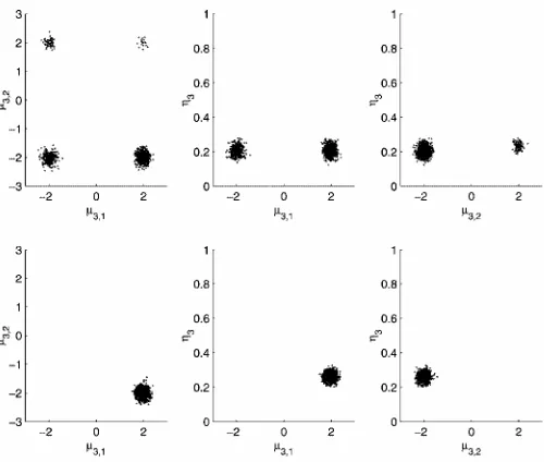
Figure 4. Modeling the Empirical Data by a Three-Groups Model; Simulations of the Group-Specic Means From the Unconstrained Posterior.
large number of groupsKand high-dimensionalparameter vec-tors, suggests that as long as the data supports the number of groups chosen for the model, a graphical inspection of the pos-terior will lead to constraints that identify a unique labeling. When there are many groups, the identication of a unique la-beling proceeds sequentially. Usually, there is one parameter or an easily identied linear combination of very few parameters that divides the posterior into two subsets containing several groups each. Conditional on this rst restriction, each subset is investigated in turn for an additional restriction that identi-es even smaller subsets of groups until nally every group is identied. Note, however, that any suitable constraint is only an indirect devise to identify a unique labeling, and therefore is not necessarily unique. (For more details, see the case studies in Schnatter 2001a,b, and Kaufmann and Frühwirth-Schnatter 2002.) For an identication problem that was more challenging due to the higher number of classes, Otter, Tüchler, and Frühwirth-Schnatter (2002) identied a latent class model with nine classes for the present case study. Alternative ap-proaches to identify a unique labeling have been discussed by Celeux et al. (2000) and Stephens (2000).
Tüchler, Frühwirth-Schnatter, and Otter (2002) reported that Bayesian model choice criteria indicated that the optimal model in the model class with homogeneous error variances and xed quadratic price interactions has three groups. For this model, we explore simulations from the unconstrained posterior to nd an (not necessarily unique) identiability constraint (Fig. 4). From this plot, we can readily identify the three simulation clusters and can easily make out an identiability constraint, namelyR: price1<min.price2;3), to separate the rst group from the other two, and RQ2>RQ3to distinguish between the two remaining
groups. The simulations of the constrained posterior resulting when applying this constraint are plotted in Figure 5.
Figure 6 shows the posterior simulations for a model with KD4 groups and xed quadratic price interactions. From this plot, it is obvious that the data support only three simulation clusters. The fourth group is spread over the parameter space, and therefore this plot can be used as an empirical indicator for determining the optimal number of groupsKD3.
Figure 5. Modeling the Empirical Data by a Three-Group Model; Simulations of the Group-Specic Means From the Constrained Posterior.
Figure 6. Modeling the Empirical Data by a Four-Group Model; Sim-ulations of the Group-Specic Means From the Unconstrained Posterior.
4.3 Comparison of the Three Algorithms and the Two Parameterizations
To investigate the inuence of the two types of parameter-ization on Algorithm 1 (full conditional Gibbs sampling) and on Algorithm 2 (partially marginalized Gibbs sampling), we choose a model with two groups and xed quadratic price inter-action effects. We did not use the three-group model with xed quadratic interactions in this comparison because Algorithm 1’s behavior in combination with the noncentered parameterization is extraordinarily bad in this case. It was not possible to sam-ple the optimal three-group model with xed quadratic interac-tions with this algorithm. This is illustrated in Figure 7, which shows marginal densities of the group weights for the optimal three-group model. Figure 7a indicates that Algorithm 1 (cen-tered), Algorithm 2, and Algorithm 3 estimate group sizes´of approximately .47, .43, and .1. In sharp contrast, we see from Figure 7b that Algorithm 1 with thenoncentered parameteriza-tion samples two groups of size .59 and .41 and a third group of size close to 0. This has a considerable inuence on model estimation. If we estimated our empirical data just with Algo-rithm 1 in combination with the noncentered parameterization the marginal densities of the group weights plotted on the right side of Figure 7 would suggest that a three-group model is a model with too high a number of groups, and we would end up with a model with fewer groups.
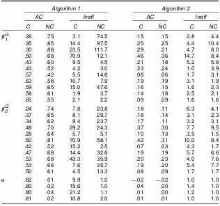
For the two-group model with xed quadratic interactions the MCMC samples obtained from Algorithms 1 and 2 under the two different parameterizations are again compared by their lag 1 sample autocorrelations and the inefciency factors. The values are listed in Table 4 for the group-specic means ¯Gk
and xed effects ®. We see that Algorithm 2 behaves invari-antly with regard to the parameterization. For Algorithm 1, the behavior is two fold. For the group-specic means¯Gk, the centered parameterization is preferred, whereas for the xed ef-fects®, the noncentered parameterization turns out to be better, so we cannot decide which parameterization to choose. In ad-dition, the results of Table 4 clearly advocate for choosing Al-gorithm 2, because nearly all autocorrelations and inefciency
(a)
(b)
Figure 7. Marginal Densities of the Group-Weights´When Applying the Model With Three Groups and Fixed Quadratic Interactions to the Empirical Data. [(a)-¢-¢-¢-, Algorithm 1, centered; - - - - -, Algorithm 2, centered; – – – – –, Algorithm 2, noncentered;¢ ¢ ¢ ¢ ¢ ¢, Algorithm 3, cen-tered. (b) -¢-¢-¢-, Algorithm 1, noncentered.]
factors lead to better values for Algorithm 2 than for Algo-rithm 1 regardless of the parameterization.
As in the simulation studies, it again turned out that ap-plying Algorithm 3’s Metropolis–Hastings steps to sample the group-specic covariancesQG1; : : : ;QGK does not improve the sampler’s autocorrelation and efciency in comparison to Al-gorithm 2. However, sampling the model error variance¾"2with Algorithm 3’s Metropolis–Hastings steps improves the quality of the sampler. The autocorrelation at lag 1 is .62 for Algo-rithm 2 and .16 for AlgoAlgo-rithm 3, and the inefciency factor de-creases from 6.5 to 1.0.
5. CONCLUDING REMARKS
In this article we tried to provide a deeper understanding of the circumstances under which full conditional Gibbs sampling of the heterogeneity model will be a sensible tool for Bayesian estimation. It turned out that full conditional Gibbs sampling is sensitive to the parameterization used for the mean, and we demonstrated that the best thing one could do for a model with anormalobservation density is to use an at least partly mar-ginalized sampler where the random effects are integrated out.
Table 4. Empirical Study, Model With Two Groups and Fixed Quadratic Interactions, Autocorrelation at Lag 1 (AC) and Inefciency Factors (Ineff) for Algorithms 1 and 2
With the Centered (C) and the Noncentered (NC) Parameterization
Algorithm 1 Algorithm 2
AC Ineff AC Ineff
C NC C NC C NC C NC
¯G1 .26 .75 3.1 74.5 .15 .15 2.8 4.4
.35 .85 14.4 97.5 .25 .25 4.4 10.4 .30 .88 23.5 111.7 .29 .21 4.7 8.0 .50 .68 70.9 12.1 .46 .36 14.7 8.4 .43 .60 9.5 4.5 .21 .18 5.2 5.8 .43 .52 4.2 3.0 .23 .24 1.0 3.9 .57 .42 5.5 14.8 .06 .06 1.7 3.1 .63 .58 10.7 7.9 .19 .19 3.1 1.9 .59 .65 15.0 47.6 .16 .15 1.6 2.3 .58 .61 1.9 3.7 .14 .18 2.5 2.1 .65 .55 2.1 2.2 .09 .09 1.6 1.6
¯G2 .24 .74 7.8 23.8 .18 .11 6.3 4.1
.37 .65 8.1 29.7 .18 .14 3.1 2.3 .34 .62 9.4 23.7 .17 .11 3.2 3.1 .48 .70 29.2 24.3 .37 .30 7.7 9.5 .28 .64 5.7 5.1 .10 .13 3.5 1.5 .50 .81 70.9 58.1 .42 .31 10.0 8.4 .42 .52 15.2 2.5 .07 .03 4.3 1.7 .47 .68 14.4 32.8 .19 .19 5.7 6.6 .53 .68 43.3 35.9 .20 .23 4.0 7.6 .53 .66 7.6 35.7 .19 .20 5.4 7.7 .50 .61 4.5 13.3 .08 .09 1.7 1.7
® .82 .01 9.9 1.0 ¡.02 ¡.02 1.0 1.0
.80 .02 15.6 1.0 .04 .00 1.4 1.0 .80 .04 21.2 1.1 .01 .00 1.2 1.0 .81 .02 10.8 2.0 .01 .01 1.0 1.0
Marginalization is usually not possible for models with non-normal observation densities and understanding full conditional Gibbs sampling is even more important for this case. Although we did not investigate nonnormal models, we believe that the results presented here will generalize to this case.
A limitation of this article is that we studied only the ef-fect of the parameterization of the mean on the performance of full conditional Gibbs sampling. An additional and equally im-portant issue that we did not investigate is how parameterizing the variance structure inuences the efciency of the MCMC sampler. From Tables 1 and 2, we hypothesize that the current method for parameterizing the variance structure is rather ef-cient, if the variances are not too small. In the case of small vari-ances using the parameterization that is centered in the mean around0(“noncentered”in the terminology of the article) helps improve the efciency of estimating the mean parameters, but does not seem to improve the efciency of variance parame-ters estimation. How to improve the estimation of variances in cases of small variances remains to be investigated, however. Meng and Van Dyck (1998) and Van Dyck and Meng (2001) explored a parameterization where the variance of the random effects is centered around the standard covariance matrix equal to the identity matrixIfor random coefcient models. Extend-ing their ideas to mixture of random-effects models yields
yiDX1i®CX
2
i¯ G k CX
2
i.Q G k/
1=2z
iC"i; ifSiDk; and
zi»N.0;I/; iD1; : : : ;N;
with the random effects centered aroundIinstead ofQSi. We leave the investigation of this parameterization to future re-search, however.
ACKNOWLEDGMENTS
This research was supported by the Austrian Science Foun-dation (FWF) under grant SFB 010 (Adaptive Information Sys-tems and Modeling in Economics and Management Science).
APPENDIX A: THE PRIOR
The following prior information was used in the estimation:
² We impose the following prior on the effects for the cen-tered parameterization. We assume that the group-specic effects¯G1; : : : ;¯GK are a priori independently identically distributed with¯Gk »N.c0;C0/forkD1; : : : ;K, whereas
the xed effects ®are a priori normally distributed with
®»N.a0;A0/. This prior must be transformed to obtain
the prior under the noncentered parameterization.
² The group-specic covariancesQG1; : : : ;QGKare a priori in-dependentlyidentically distributed withQGk »IW.º0Q;SQ0/. ² The probability distribution of´follows a Dirichlet prior,
D.e0;1; : : : ;e0;K/.
² The observation equation’s variance¾"2is a priori inverted-gamma distributed withIG.º";0;S";0/.
In the empirical study of Section 4 c0 anda0are the
ordi-nary least squares (OLS) estimates obtained by a model with
xed effects only.C0andA0are diagonal matrices with
diag-onal elements equal to 25. We select ºQ0 D10. SQ0 is derived from the relationshipE.QGk/D.ºQ0 ¡.dC1/=2/¡1SQ0, where E.QGk/was computed by individual OLS estimation and d is the dimensionality ofQGk. We selecte0;kD1 forkD1; : : : ;K, which leads to a uniform prior on the unit simplex, and we stay fully noninformative about¾"2.
APPENDIX B: DETAILS OF ALGORITHM 2
B.1 Sampling.ÁL,¯N/by a Blocked Gibbs Sampler
We give details only for the centered parameterization. The conditional posterior ofÁLand¯N partitions as
¼.ÁL;¯NjyN;ÁV;SN/
The conditionalposterior of the random effects¯iis the normal distribution¼.¯ijyi;ÁL;ÁV;Si/»N.¯GSiC Obi;Bi/with sider the marginal model from (13) with the random effects integrated out. An alternative way to write this model is
yiDZ¤i®¤C"¤i; "¤i »N.0;Vi/; (B.1)
From the marginal model (B.1), we see that the poste-rior of ÁL is normally distributed with ¼.ÁLjyN;ÁV;SN/»
Here ÁL may be sampled directly from (B.2) and (B.3). The information matrix .A¤N/¡1, however, has a special structure
that can be exploited for efcient sampling. If no xed ef-fects®are present, then.A¤N/¡1 andA¤N are block diagonal, and we may sample all group-specic effects independently. If xed effects ® are present, then .A¤N/¡1 and A¤N contain a submatrix that is block diagonal. Therefore, joint sampling of ÁL D.®;¯G1; : : : ;¯GK/ is possible by sampling the xed effects from the marginal posterior N.cN;CN/, where the group-specic effects are integrated out, and by sampling the group-specic effects independently from the conditional dis-tributions N.bN;k.®/;BN;k/;k D1; : : : ;K. The moments of these densities are given by
bN;k.®/DBN;k
Applying Bayes’ theorem, we obtain
¼.SNjyN;Á//
Therefore, S1; : : : ;SN are conditionally independent given
ÁandyN, and we sampleSi foriD1; : : : ;Nfrom the discrete distribution
¼.SiDkjyi;Á//L.yij®;¯Gk;QGk; ¾"2/¢´k: (B.4)
To obtain the likelihood, we use the marginal model (13) where the random effects are integrated out. Therefore, the likelihood in (B.4) is the likelihood of the normal distributionN.yiIX1i®C
X2i¯Gk;X2iQGk.X2i/0C¾"2I/.
B.3 Sampling the Variance Parameters
Although sampling the variance parametersÁV D.QG1; : : : ;
QGK; ¾"2/ conditional on ¯N, ÁL, SN, and yN is identical to the corresponding step in Algorithm 1 applied by Lenk and DeSarbo (2000), we give details here as a matter of refer-ence. Conditional on ¯N, ÁL, SN, and yN, the parameters
QG1; : : : ;QGK; ¾"2are pairwise independent.The conditionalpos-terior ofQGk given¯N,ÁL,SN, andyN is an inverted Wishart
density being independent ofyNand all group-specic
parame-APPENDIX C: DETAILS OF ALGORITHM 3
Here we give details on how to sample the variance parame-ters.QG1; : : : ;QGK; ¾"2/conditional onÁL,SN,yN within step Metropolis–Hastings algorithm. Let .QGk/old be the current value ofQGk. We sample a new covariance matrix.QGk/newfrom
To compute the ratio, we use the facts that the posterior
¼.QG1; : : : ;QGK; ¾"2jÁL;SN;yN/ is proportional to the quantity in (14) and that the unknown normalizing constant cancels.
The design of a suitable proposal density turned out to be somewhat challenging. We use a mixture of inverted Wishart proposal,
given that the random effects are equal to.¯N/j. This posterior is an inverted Wishart density and appeared both in Algorithm 1 and Algorithm 2 [see (B.5)]..¯N/jin (C.2) is sampled from the
conditionalposterior¼.¯NjÁL;SN; .QGk/old;QG¡k; ¾"2;yN/. The rationale behind this choice is that asJ! 1, the proposal ap-proaches the conditionalmarginal posterior¼.QGkjQ¡Gk; ¾"2;ÁL;
SN;yN/that we require to sample from.
The posterior ¼.¯NjÁL;SN; .QGk/old;QG¡k; ¾"2;yN/ is the same as in step (iii-3b) of this algorithm. Therefore, to ob-tain.¯N/j,jD1; : : : ;J, we repeat step (iii-3b)Jtimes to con-struct the proposal densityq.QGkj.QkG/old/. To sample.QGk/new
fromq.QGkj.QGk/old/, we rst randomly select a componentQj, and then sample.QGk/newfrom the conditionalinverted Wishart density ¼.QGkj.¯N/Qj;¯Gk;SN/. Note that for evaluating q..QGk/oldj.QGk/new/ in the acceptance ratio (C.1), we need to sample furtherJ values .¯N/j from the conditional pos-terior¼.¯NjÁL;SN; .QGk/new;QG¡k; ¾"2;yN/, where the covari-ance matrix of groupkis substituted by.QGk/new. IncreasingJ will increase the acceptance rate of the Metropolis–Hastings al-gorithm; however, choosingJtoo large will slow the algorithm, because for each step and each group we need 2J functional evaluations of an inverted Wishart density.
A comparable Metropolis–Hastings algorithm is used to sample¾"2.
APPENDIX D: PROOF OF (21)
Equation (21) is easy to verify. First,
EA alllands, and the following holds:
EA strained to the labeling subspace L l, is related to the un-constrained posterior¼.ÃjyN/ by ¼Ll.ÃjyN/DK!¼.ÃjyN/. Therefore, (21) follows from (D.1),
EA
[Received May 2000. Revised May 2003.]
REFERENCES
Aitkin, M., and Rubin, D. B. (1985), “Estimation and Hypothesis Testing in Finite Mixture Models,”Journal of the Royal Statistical Society, Ser. B, 47, 67–75.
Allenby, G. M., Arora, N., and Ginter, J. L. (1998), “On the Heterogeneity of Demand,”Journal of Marketing Research, 35, 384–389.
Celeux, G., Hurn, M., and Robert, C. P. (2000), “Computational and Inferential Difculties with Mixture Posterior Distributions,”Journal of the American Statistical Association, 95, 957–970.
Chen, M., Shao, Q., and Ibrahim, J. (2000),Monte Carlo Methods in Bayesian Computation, New York: Springer.
Chib, S., and Carlin, B. (1999), “On MCMC Sampling in Hierarchical Longi-tudinal Models,”Statistics and Computing, 9, 17–26.
Elrod, T., Louviere, J. J., and Davey, K. S. (1992), “An Empirical Comparison of Ratings-Based and Choice-Based Conjoint Models,”Journal of Marketing Research, 29, 368–377.
Frühwirth-Schnatter, S. (1999), “Model Likelihoods and Bayes Factors for Switching and Mixture Models,” preprint, Vienna University of Economics and Business Administration, revised version submitted for publication.
(2001a), “Markov Chain Monte Carlo Estimation of Classical and Dy-namic Switching and Mixture Models,”Journal of the American Statistical Association,96, 194–209.
(2001b), “Fully Bayesian Analysis of Switching Gaussian State-Space Models,”Annals of the Institute of Mathematical Statistics, 53, 31–49. Frühwirth-Schnatter, S., and Otter, T. (1999), “Conjoint Analysis Using Mixed
Effect Models,” inStatistical Modelling, Proceedings of the Fourteenth In-ternational Workshop on Statistical Modelling, eds. H. Friedl, A. Berghold, and G. Kauermann, Graz, pp. 181–191.
Gelfand, A. E., Sahu, S. K., and Carlin, B. P. (1995), “Efcient Parameteriza-tions for Normal Linear Mixed Models,”Biometrika, 82, 479–488. Gerlach, R., Carter, C., and Kohn, R. (2000), “Efcient Bayesian Inference for
Dynamic Mixture Models,”Journal of the American Statistical Association, 95, 819–828.
Geweke, J. (1992), “Evaluating the Accuracy of Sampling-Based Approaches to the Calculation of Posterior Moments,” inBayesian Statistics (Vol. 4), eds. J. M. Bernardo, J. O. Berger, A. P. Dawid, and A. F. M. Smith, Oxford, U.K.: Oxford University Press, pp. 169–193.
Kaufmann, S., and Frühwirth-Schnatter, S. (2002), “Bayesian Analysis of Switching ARCH Models,”Journal of Time Series Analysis, 23, 425–458. Lenk, P. J., and DeSarbo, W. S. (2000), “Bayesian Inference for Finite Mixture
of Generalized Linear Models With Random Effects,”Psychometrika, 65, 93–119.
Liu, J., Wong, W., and Kong, A. (1994), “Covariance Structure of the Gibbs Sampler With Applications to the Comparisons of Estimators and Augmen-tation Schemes,”Biometrika, 81, 27–40.
Meng, X., and Van Dyck, D. (1998), “Fast EM-Type Implementations for Mixed Effects Models,”Journal of the Royal Statistical Society, Ser. B, 60, 559–578.
Otter, T., Tüchler, R., and Frühwirth-Schnatter, S. (2002), “Bayesian Latent Class Metric Conjoint Analysis—A Case Study from the Austrian Mineral Water Market,” inExplanatory Data Analysis in Empirical Research, eds. O. Opitz and M. Schwaiger, Berlin: Springer-Verlag, pp. 157–169. Stephens, M. (2000), “Dealing With Label Switching in Mixture Models,”
Jour-nal of the Royal Statistical Society, Ser. B, 62, 795–809.
Tüchler, R., Frühwirth-Schnatter, S., and Otter, T. (2002), “The Heterogene-ity Model and Its Special Cases—An Illustrative Comparison,” in Pro-ceedings of the 17th International Workshop on Statistical Modelling, eds. M. Stasinopoulos and G. Touloumi, Chania, Greece, pp. 637–644. Van Dyck, D., and Meng, X. (2001), “The Art of Data Augmentation,”Journal
of Computational and Graphical Statistics,110, 1–50.
Verbeke, G., and Lesaffre, E. (1996), “A Linear Mixed-Effects Model With Heterogeneity in the Random-Effects Population,”Journal of the American Statistical Association, 91, 217–221.
Verbeke, G., and Molenberghs, G. (2000),Linear Mixed Models for Longitudi-nal Data, New York: Springer.