Full Terms & Conditions of access and use can be found at
http://www.tandfonline.com/action/journalInformation?journalCode=ubes20 Download by: [Universitas Maritim Raja Ali Haji], [UNIVERSITAS MARITIM RAJA ALI HAJI
TANJUNGPINANG, KEPULAUAN RIAU] Date: 11 January 2016, At: 20:59
Journal of Business & Economic Statistics
ISSN: 0735-0015 (Print) 1537-2707 (Online) Journal homepage: http://www.tandfonline.com/loi/ubes20
Testing the Unconfoundedness Assumption via
Inverse Probability Weighted Estimators of (L)ATT
Stephen G. Donald, Yu-Chin Hsu & Robert P. Lieli
To cite this article: Stephen G. Donald, Yu-Chin Hsu & Robert P. Lieli (2014) Testing the
Unconfoundedness Assumption via Inverse Probability Weighted Estimators of (L)ATT, Journal of Business & Economic Statistics, 32:3, 395-415, DOI: 10.1080/07350015.2014.888290
To link to this article: http://dx.doi.org/10.1080/07350015.2014.888290
View supplementary material
Accepted author version posted online: 10 Mar 2014.
Submit your article to this journal
Article views: 204
View related articles
View Crossmark data
Testing the Unconfoundedness Assumption via
Inverse Probability Weighted Estimators
of (L)ATT
Stephen G. D
ONALDDepartment of Economics, University of Texas, Austin, TX 78712 ([email protected])
Yu-Chin H
SUInstitute of Economics, Academia Sinica, Taipei, Taiwan ([email protected])
Robert P. L
IELIDepartment of Economics, Central European University, Budapest and Magyar Nemzeti Bank, Budapest, Hungary ([email protected])
We propose inverse probability weighted estimators for the local average treatment effect (LATE) and the local average treatment effect for the treated (LATT) under instrumental variable assumptions with covariates. We show that these estimators are asymptotically normal and efficient. When the (binary) instrument satisfies one-sided noncompliance, we propose a Durbin–Wu–Hausman-type test of whether treatment assignment is unconfounded conditional on some observables. The test is based on the fact that under one-sided noncompliance LATT coincides with the average treatment effect for the treated (ATT). We conduct Monte Carlo simulations to demonstrate, among other things, that part of the theoretical efficiency gain afforded by unconfoundedness in estimating ATT survives pretesting. We illustrate the implementation of the test on data from training programs administered under the Job Training Partnership Act in the United States. This article has online supplementary material.
KEY WORDS: Instrumental variables; Inverse probability weighted estimation; Local average treatment effect; Nonparametric estimation.
1. INTRODUCTION
Nonparametric estimation of average treatment effects (ATEs) from observational data is typically undertaken under one of two types of identifying conditions. The unconfounded-ness assumption, in its weaker form, postulates that treatment assignment is mean-independent of potential outcomes con-ditional on a vector of observed covariates. This requirement carries with it considerable identifying power; specifically, it identifies the ATE and the average treatment effect for the treated (ATT) without any additional modeling assumptions. On the other hand, if unobserved confounders exist, then instrumen-tal variables—related to the outcome only through changing the likelihood of treatment—are typically used to learn about treatment effects. Without further assumptions, the availabil-ity of an instrumental variable (IV) is, however, not sufficient to identify ATE or ATT. In general, the IV will identify only the local average treatment effect (LATE; Imbens and Angrist 1994) and the local average treatment effect for the treated (LATT; Fr¨olich and Lechner2010; Hong and Nekipelov2010). If one specializes to binary instruments, as we do in this article, then the LATE and LATT parameters correspond to the ATE over specific subgroups of the population. These subgroups are, however, dependent on the choice of the instrument and are gen-erally unobserved. Partly for these reasons a number of authors have called into question the usefulness of LATE for program evaluation (Heckman1997; Deaton2009; Heckman and Urz´ua 2010). In most such settings, ATE and ATT are more natural and practically relevant parameters of interest—provided that they
can be credibly identified and accurately estimated. (In fairness, some of the criticism in Deaton (2009) goes beyond LATE, and also applies to ATE/ATT as a parameter of interest. See Imbens (2010) for a response to Deaton (2009).)
When using instrumental variables, empirical researchers are often called upon to tell a “story” to justify their validity. As pointed out by Abadie (2003) and Fr¨olich (2007), it is often easier to argue that the relevant IV conditions hold if condi-tioning on a vector of observed covariates is also allowed. In particular, Fr¨olich (2007) showed that in this scenario LATE is still nonparametrically identified and proposes efficient esti-mators, based on nonparametric imputation and matching, for this quantity. Given the possible need to condition on a vec-tor of observables to justify the IV assumptions, it is natural to ask whether treatment assignment itself might be unconfounded conditional on the same (or maybe a larger or smaller) vector of covariates. In this article, we propose a formal test of this hy-pothesis that relies on the availability of a specific kind of binary instrument for which LATT=ATT (so that the latter parameter is also identified). Establishing unconfoundedness under these conditions still offers at least two benefits: (i) it enables the es-timation of an additional parameter of interest (namely, ATE) and (ii) it potentially allows for more efficient estimation of ATT than IV methods (we will argue this point in more detail later).
© 2014American Statistical Association Journal of Business & Economic Statistics July 2014, Vol. 32, No. 3 DOI:10.1080/07350015.2014.888290
395
To our knowledge, this is the first test in the literature aimed at this task.
More specifically, the contributions of this work are two-fold. First, given a (conditionally) valid binary instrument, we propose alternative nonparametric IV estimators of LATE and LATT. These estimators rely on weighting by the inverse of the estimated instrument propensity score and are computed as the ratio of two estimators that are of the form proposed by Hirano, Imbens, and Ridder (2003), henceforth HIR. While Fr¨olich (2007) conjectured in passing that such an estimator of LATE should be efficient, he did not provide a proof. We fill this (admittedly small) gap in the literature and formally establish the first-order asymptotic equivalence of our LATE estimator and Fr¨olich’s imputation/matching-based estimators. We also demonstrate that our LATT estimator is asymptotically efficient, that is, first-order equivalent to that of Hong and Nekipelov (2010).
More importantly, we propose a Durbin–Wu–Hausman-type test for the unconfoundedness assumption. On the one hand, if a binary instrument satisfying “one-sided noncompliance” (e.g., Fr¨olich and Melly2013a) is available, then the LATT parameter associated with that instrument coincides with ATT, and is con-sistently estimable using the estimator we proposed. (Whether one-sided noncompliance holds is verifiable from the data.) On the other hand, if treatment assignment is unconfounded given a vector of covariates, ATT can also be consistently estimated us-ing the HIR estimator. If the unconfondedness assumption does not hold, then the HIR estimator will generally converge to a different limit. Thus, the unconfoundedness assumption can be tested by comparing our estimator of LATT with HIR’s estima-tor of ATT. Of course, if the validity of the instrument itself is questionable, then the test should be more carefully interpreted as a joint test of the IV conditions and the unconfoundedness assumption. We use a battery of Monte Carlo simulations to explore in detail the finite sample properties of our IV estimator and the proposed test statistic. We also provide an application to illustrate how to implement and interpret the test in practice. We use the dataset from Abadie, Angrist, and Imbens (2002) on training programs administered under the Job Training Partner-ship Act (JTPA) in the United States and highlight a difference between the self-selection process of men versus women into these programs.
The rest of the article is organized as follows. In Section2, we present the theoretical framework; in Section3, we describe the estimators for LATE and LATT. The implications of uncon-foundedness and the proposed test for it are discussed in Sec-tion 4. A rich set of Monte Carlo results is presented in Sec-tion 5. In Section 6, we give the empirical application along with an additional, empirically motivated, Monte Carlo exer-cise. Section7summarizes and concludes. The most important proofs and the simulation tables from Section5are collected in the Appendix. More detailed proofs and some additional simu-lations are available as an online supplement.
2. THE BASIC FRAMEWORK AND IDENTIFICATION RESULTS
The following IV framework, augmented by covariates, is now standard in the treatment effect literature; see, for
ex-ample, Abadie (2003) or Fr¨olich (2007) for a more detailed exposition. For each population unit (individual), one can ob-serve the value of a binary instrumentZ∈ {0,1}and a vec-tor of covariates X∈Rk. For Z
=z, the random variable
D(z)∈ {0,1}specifies individuals’ potential treatment status withD(z)=1 corresponding to treatment andD(z)=0 to no treatment. The actually observed treatment status is then given byD≡D(Z)=D(1)Z+D(0)(1−Z). Similarly, the random variableY(z, d) denotes the potential outcomes in the popu-lation that would obtain if one were to setZ=zandD=d
exogenously. The following assumptions, taken from Abadie (2003) and Fr¨olich (2007) with some modifications, describe the relationships between the variables defined above and jus-tifyZbeing referred to as an instrument:
Assumption 1. Let V =(Y(0,0), Y(0,1), Y(1,0), Y(1,1), D(1), D(0))′.
(i) (Moments):E(V′V)<∞.
(ii) (Instrument assignment): There exists a subset X1 of X
such thatE(V|Z, X1)=E(V|X1) andE(V V′|Z, X1)=
E(V V′|X
1) a.s. inX1.
(iii) (Exclusion of the instrument):P[Y(1, d)=Y(0, d)]=1 ford ∈ {0,1}.
(iv) (First stage): P[D(1)=1]> P[D(0)=1] and 0< P(Z=1|X1)<1 forX1defined in (ii).
(v) (Monotonicity):P[D(1)≥D(0)]=1.
Assumption 1(i) ensures the existence of the moments we will work with. Part (ii) states that, conditional on X1, the
instrument is exogenous with respect to the first and second moments of the potential outcome and treatment status vari-ables. This is satisfied, for example, if the value of the in-strument is completely randomly assigned or the inin-strument assignment is independent ofV conditional on X1.
Neverthe-less, part (ii) is weaker than the full conditional independence assumed in Abadie (2003) and Fr¨olich (2007), but is still suf-ficient for identifying LATE and LATT. Part (iii) precludes the instrument from having a direct effect on potential outcomes. Part (iv) postulates that the instrument is (positively) related to the probability of being treated and implies that the distributions
X1|Z=0 and X1|Z=1 have common support. Finally, the
monotonicity ofD(z) inz, required in part (v), allows for three different types of population units with nonzero mass: compli-ers [D(0)=0, D(1)=1], always takers [D(0)=1, D(1)=1] and never takers [D(0)=0, D(1)=0] (see Imbens and Angrist 1994). Of these, compliers are actually required to have posi-tive mass—part (iv) rules outP[D(1)=D(0)]=1. In light of these assumptions, it is customary to think ofZas a variable that indicates whether an exogenous incentive to obtain treatment is present or as a variable signaling “intention to treat.”
Given the exclusion restriction in part (iii), one can sim-plify the definition of the potential outcome variables as
Y(d)≡Y(1, d)=Y(0, d),d=0,1. The actually observed out-comes are then given byY ≡Y(D)=Y(1)D+Y(0)(1−D). The LATE (≡τ) and LATT (≡τt) parameters associated with
the instrumentZare defined as
τ ≡E[Y(1)−Y(0)|D(1)=1, D(0)=0], τt ≡E[Y(1)−Y(0)|D(1)=1, D(0)=0, D=1].
LATE, originally due to Imbens and Angrist (1994), is the ATE in the complier subpopulation. The LATT parameter was con-sidered, for example, by Fr¨olich and Lechner (2010) and Hong and Nekipelov (2010). LATT is the ATE among those compliers who actually receive the treatment. Of course, in the subpopu-lation of compliers the conditionD=1 is equivalent toZ=1, that is, LATT can also be written asE[Y(1)−Y(0)|D(1)= 1, D(0)=0, Z=1]. In particular, if Z is an instrument that satisfies Assumption 1 unconditionally (sayZis assigned com-pletely at random), then LATT coincides with LATE. Our in-terest in LATT is motivated mainly by the fact that it can serve as a bridge between the IV assumptions and unconfoundedness (this connection will be developed shortly).
Under Assumption 1 one can also interpret LATE/LATT as the ATE/ATT ofZ onY divided by the ATE/ATT of Z onD. More formally, defineW(z)≡D(z)Y(1)+(1−D(z))Y(0) and
W ≡W(Z)=ZW(1)+(1−Z)W(0). It is easy to verify that
W =DY(1)+(1−D)Y(0)=Y and
τ =E[W(1)−W(0)]/E[D(1)−D(0)] (1)
τt =E[W(1)−W(0)|Z=1]/E[D(1)−D(0)|Z=1].
(2)
The quantities on the right-hand side of (1) and (2) are non-parametrically identified from the joint distribution of the ob-servables (Y, D, Z, X1). We denote the conditional
probabil-ityP(Z=1|X1) byq(X1) and refer to it as the “instrument
propensity score” to distinguish it from the conventional use of the term propensity score (the conditional probability of be-ing treated). Under Assumption 1, the followbe-ing identification results are implied, for example, by Theorem 3.1 in Abadie (2003):
E[W(1)−W(0)]=E
ZY q(X1)−
(1−Z)Y
1−q(X1)
≡ (3)
E[D(1)−D(0)]=E
ZD q(X1)−
(1−Z)D
1−q(X1)
≡Ŵ (4)
E[W(1)−W(0)|Z=1]
= E
q(X1)
ZY
q(X1)−
(1−Z)Y
1−q(X1)
E[q(X1)]≡t
(5)
E[D(1)−D(0)|Z=1]
= E
q(X1)
ZD
q(X1)−
(1−Z)D
1−q(X1)
E[q(X1)]≡Ŵt.
(6)
That is,τ =/ Ŵandτt =t/ Ŵt.
The unconfoundedness assumption, introduced by Rosen-baum and Rubin (1983), is also known in the literature as selection-on-observables, conditional independence, or
ignor-ability. We say that treatment assignment is unconfounded con-ditional on a subsetX2of the vectorXif
Assumption 2 (Unconfoundedness). Y(1) andY(0) are mean-independent ofDconditional onX2, that is,E[Y(d)|D, X2]=
E[Y(d)|X2],d ∈ {0,1}.
Assumption 2 is stronger than Assumption 1 in that it rules out unobserved factors related to the potential outcomes playing a systematic role in selection to treatment. Furthermore, it permits nonparametric identification of ATE=E[Y(1)−Y(0)] as well as ATT=E[Y(1)−Y(0)|D=1]. For example, ATE and ATT can be identified by expressions analogous to (3) and (4), respec-tively: replaceZwithDandq(X1) withp(X2)=P(D=1|X2).
(The conditionE[Y(0)|D, X2]=E[Y(0)|X2] is actually
suffi-cient for identifying ATT.)
As mentioned above, ATE and ATT are often of more in-terest to decision makers than local treatment effects, but are not generally identified under Assumption 1 alone. A partial exception is when the instrumentZ satisfies a strengthening of the monotonicity property called one-sided noncompliance (see, e.g., Fr¨olich and Melly2013a):
Assumption 3 (One-sided noncompliance). P[D(0)= 0]=1.
Assumption 3 dates back to (at least) Bloom (1984), who estimated the effect of a program in the presence of “no shows.” The stated condition means that those individuals for whom
Z=0 are excluded from the treatment group, while those for whom Z=1 generally have the option to accept or decline treatment. Hence, there are no always-takers; noncompliance with the intention-to-treat variable Z is only possible when
Z=1. More formally, for such an instrumentD=ZD(1), and soD=1 impliesD(1)=1 (the treated are a subset of the com-pliers). Therefore,
LATT=E[Y(1)−Y(0)|D(1)=1, D(0)=0, D=1] =E[Y(1)−Y(0)|D(1)=1, D=1]
=E[Y(1)−Y(0)|D=1]=ATT. (7) Thus, under one-sided noncompliance, ATT=LATT. The ATE parameter, on the other hand, remains generally unidentified under Assumptions 1 and 3 alone.
In Section4, we will show how one can test Assumption 2 when a binary instrument, valid conditional onX1and
satisfy-ing one-sided noncompliance, is available. Fr¨olich and Lechner (2010) also considered some consequences for identification of the IV assumption and unconfoundedness holding simulta-neously (without one-sided noncompliance), but they did not discuss estimation by inverse probability weighting, propose a test, or draw out implications for efficiency.
3. THE ESTIMATORS AND THEIR ASYMPTOTIC PROPERTIES
3.1 Inverse Propensity Weighted Estimators of LATE and LATT
Let {(Yi, Di, Zi, X1i)}ni=1 denote a random sample of
ob-servations on (Y, D, Z, X1). The proposed inverse probability
weighted (IPW) estimators forτ andτt are based on sample
where ˆq(·) is a suitable nonparametric estimator of the instru-ment propensity score function. If there are no covariates in the model, then both ˆτ and ˆτtreduce to
which is the LATE estimator developed in Imbens and Angrist (1994) and is also known as the Wald estimator, after Wald (1940).
Following HIR, we use the series logit estimator (SLE) to estimate q(·). The first-order asymptotic results presented in Section3.2do not depend critically on this choice—the same conclusions could be obtained under similar conditions if other suitable estimators of q(·) were used instead. For example, Ichimura and Linton (2005) used local polynomial regression and Abrevaya, Hsu, and Lieli (2013) used higher order kernel regression. We opt for the SLE for three reasons: (i) it is au-tomatically bounded between zero and one; (ii) it allows for a more unified treatment of continuous and discrete covariates in practice; (iii) the curse of dimensionality affects the imple-mentability of the SLE less severely. (We do not say that the SLE is immune to dimensionality; however, if one uses, say, higher order local polynomials andX1is large, then one either
needs a very large bandwidth or an astronomical number of ob-servations just to be able to compute each ˆq(X1i), at least if the
kernel weights have bounded support. A sufficiently restricted version of the SLE is always easy to compute.)
We implement the SLE using power series. Let λ=
(λ1, . . . , λr)′∈Nr0 be an r-dimensional vector of
nonnega-tive integers where r is the dimension of X1. Define a norm
for λ as |λ| =rj=1λj, and for x1∈Rr, let x1λ=
nondecreasing in k. For any integer K >0, define RK(x 1)=
The asymptotic properties of ˆq(x1) are discussed in Appendix
A of HIR.
3.2 First-Order Asymptotic Results
We now state conditions under which ˆτ and ˆτt are √n
-consistent, asymptotically normal and efficient.
Assumption 4 (Distribution ofX1). (i) The distribution of the
r-dimensional vector X1 is absolutely continuous with
prob-ability density f(x1); (ii) the support of X1, denoted X1, is
a Cartesian product of compact intervals; (iii) f(x1) is twice
continuously differentiable, bounded above, and bounded away from 0 onX1.
Though standard in the literature, this assumption is restric-tive in that it rules out discrete covariates. This is mostly for ex-positional convenience; after stating our formal result, we will discuss how to incorporate discrete variables into the analysis.
Next, we impose restrictions on various conditional moments ofY,D, andZ. We definemz(x1)=E[Y |X1=x1, Z=z] and
μz(x1)=E[D|X1=x1, Z=z]. Then:
Assumption 5 (Conditional Moments ofY and D). mz(x1)
andμz(x1), are continuously differentiable overX1forz=0,1.
Assumption 6 (Instrument Propensity Score). (i)q(x1) is
con-tinuously differentiable of order ¯q ≥7·r; (ii)q(x1) is bounded
away from zero and one onX1.
The last assumption specifies the estimator used for the in-strument propensity score function.
Assumption 7 (Instrument Propensity Score Esti-mator). q(x1) is estimated by SLE with a power series
satisfyingK=a·nνfor some 1/(4( ¯q/r
−1))< ν <1/9 and
a >0.
Ifq(x1) is instead estimated by local polynomial regression
or higher order kernel regression, then it is sufficient to assume less smoothness; specifically,q(x1) must be continuously
differ-entiable only of order ¯q > rfor the theoretical results to hold. The first-order asymptotic properties of ˆτ and ˆτt are stated in
the following theorem.
Theorem 1 (Asymptotic properties ofτˆandτˆt): Suppose that
Assumption 1 and Assumptions 4 through 7 are satisfied. Then,
(a) √n( ˆτ −τ)→d N(0,V) and √n( ˆτt−τt)→d N(0,Vt),
ψt(y, d, z, x1)
(b) Vis the semiparametric efficiency bound for LATE with
or without the knowledge ofq(x1);
(c) Vtis the semiparametric efficiency bound for LATT
with-out the knowledge ofq(x1).
Comments1. The result on ˆτ is analogous to Theorem 1 of HIR; the result on ˆτtis analogous to Theorem 5 of HIR. Theorem
1 shows directly that the IPW estimators of LATE and LATT presented in this article are first-order asymptotically equiva-lent to the matching/imputation based estimators developed by Fr¨olich (2007) and Hong and Nekipelov (2010).
2. Theorem 1 follows from the fact that, under the conditions stated, ˆτ and ˆτt can be expressed as asymptotically linear with
influence functionsψandψt, respectively:
√
These representations are developed in Appendix A, along with the rest of the proof.
3. To use Theorem 1 for statistical inference, one needs con-sistent estimators forVandVt. Such estimators can be obtained
by constructing uniformly consistent estimates forψandψtand
then averaging the squared estimates over the sample observa-tions{(Yi, Di, Zi, X1i)}ni=1. To be more specific, let ˆm1(x1) and
estimators. (The estimators forŴandŴt are the denominators
of ˆτ and ˆτt, respectively.) Finally, let
4. In part (b), the semiparametric efficiency bound forτ is given by Fr¨olich (2007) and Hong and Nekipelov (2010). In particular, the bounds are the same with or without the knowl-edge of the instrument propensity score functionq(x1). If the
instrument propensity score function is known, τ can also be consistently estimated by using the true instrument propensity score throughout in the formula for ˆτ. Denote this estimator by ˆτ∗. Using Remark 2 of HIR, the asymptotic variance of √
It can be shown that V ≤V∗. Therefore, the IPW estimator forτ based on the true instrument propensity score function is less efficient than that based on estimated instrument propensity score function.
5. In part (c), the semiparametric efficiency bound forτt
with-out knowledge of the instrument propensity score function is de-rived in Hong and Nekipelov (2010). The efficiency bound for
τt with knowledge of the instrument propensity score function
has not been given in the literature yet. However, by Corollary 1 and Theorem 5 of HIR, the semiparametrically efficient IPW estimator forτt is given by
ˆ
t,se≤Vt, that is, knowledge of the instrument
propensity score allows for more efficient estimation ofτt. On
the other hand, if the instrument propensity score function is known, then τt can also be consistently estimated by using
q(X1i) throughout in the formula for ˆτt,se∗ . It follows from the
discussion after Corollary 1 of HIR that ˆτtand the latter
estima-tor cannot generally be ranked in terms of efficiency.
6. Suppose thatX1 contains discrete covariates whose
pos-sible values partition the population into ¯s subpopulations or cells. Let the random variable S∈ {1, . . . ,s¯} denote the cell a given unit is drawn from. For each s one can define
q( ˜x1, s)=P(Z=1|X˜1=x˜1, S=s), where ˜X1 denotes the
continuous components ofX1, and estimate this function by SLE
on the corresponding subsample. Then LATE and LATT can be estimated in the usual way by using ˆq( ˜X1i, Si) as the instrument
propensity score (this is equivalent to computing the weighted average of the cell-specific LATE/LATT estimates). Under suit-able modifications of Assumptions 4–7, the LATE estimator so defined possesses an influence functionψ(y, d, z,x˜1, s) that
is isomorphic to ψ(y, d, z, x1); one simply replaces the
func-tions q(x1), mz(x1), μz(x1) with their cell-specific
counter-partsq( ˜x1, s),mz( ˜x1, s)=E[Y |X˜1=x˜1, S =s, Z=z], etc.
(See Abrevaya, Hsu, and Lieli (2013), Appendix D, for a formal derivation in a similar context.) However, this ap-proach may not be feasible when the number of cells is large, which is the case in many economic applications. See Com-ment 8 for restricted estimators more easily impleCom-mentable in practice.
7. The changes in the regularity conditions required by the presence of discrete variables are straightforward. For exam-ple, Assumption 4 needs to hold for the conditional distribu-tion ˜X1|S=s for any s. The functions mz( ˜x1, s), etc., need
to be continuously differentiable in ˜x for any s. Finally, in Assumptions 6 and 7, r is to be redefined as the dimension of ˜X1.
8. It is easy to specify the SLE so that it implements the sample splitting estimator described in Comment 6 above in a single step. Given a vector RK( ˜x
1) of power functions in ˜x1,
use (1{s=1}RK( ˜x1)′, . . . ,1{s=s¯}RK( ˜x1)′) in the estimation, that
is, interact the powers of ˜x1 with each subpopulation dummy.
However, if ¯s is large, the number of observations available from some of the subpopulations can be very small (or zero) even for largen. The SLE is well suited for bridging over data-poor regions using functional form restrictions. For example, one can use, for someL≤K,
that is, one only lets lower order terms vary across subpopu-lations. Alternatively, suppose thatX1=( ˜X′1, I1, I2)′whereI1
andI2are two indicators (so that ¯s=4). Then, one may
imple-ment the SLE with (RK( ˜x1)′,RK( ˜x1)′I1,RK( ˜x1)′I2), but without
RK( ˜x1)′I1I2. This constrains the attributesI1 andI2to operate
independently from each other in affecting the probability that
Z=1. Of course, the two types of restrictions can be combined. The asymptotic theory is unaffected if the restrictions are relaxed appropriately asnbecomes large (e.g.,L→ ∞whenK→ ∞
in the required manner). Furthermore, as restricting the SLE can be thought of as a form of smoothing, results by Li, Racine, and Wooldridge (2009) suggest that there might be small sample MSE gains relative to the “sample splitting” method (unless of course the misspecification bias is too large).
4. TESTING FOR UNCONFOUNDEDNESS
4.1 The Proposed Test Procedure
If treatment assignment is unconfounded conditional on a subsetX2ofX, then, under regularity conditions, one can
con-sistently estimate ATT using the estimator proposed by HIR:
ˆ
1|X2=x2), the propensity score function. More generally, let
ρd(x2)=E[Y|D=d, X2=x2] ford=0,1. Under regularity
conditions, ˆβt converges in probability toβt≡E[Y|D=1]−
E[ρ0(X2)|D=1]. If the unconfoundedness assumption holds,
thenρ0(X2)=E[Y(0)|D=1, X2], andβt reduces to ATT.
Given a binary instrument that is valid conditional on a subset
X1 of X, one-sided noncompliance implies ATT=LATT, and
hence ATT can also be consistently estimated by ˆτt. On the other
hand, if the unconfoundedness assumption does not hold, then ˆ
τt is still consistent for ATT, but ˆβtis in general not consistent
for ATT. Hence, we can test the unconfoundedness assumption (or at least a necessary condition of it) by comparing ˆτtwith ˆβt.
Assumption 4′be the analog of Assumption 4 stated forX
2;
Assumption 5′ be the analog of Assumption 5 stated for
ρd(x2),d =0,1;
Assumption 6′be the analog of Assumption 6 stated forp(x
2);
Assumption 7′be the analog of Assumption 7 stated forp(x
2),
where by “analog” we mean that all parameters are object-specific, that is, Assumption 4′ is not meant to impose, say, dim(X2)=dim(X1). The asymptotic properties of the
differ-ence between ˆτt and ˆβt are summarized in the following
theorem.
Theorem 2. Suppose that Assumption 1, Assumptions 4 through 7, and Assumptions 4′through 7′are satisfied. If, in ad-dition, σ2≡E[(ψt(Y, D, Z, X1)−φt(Y, D, X2))2]>0, then
As shown by HIR, under Assumptions 4′ through 7′ the asymptotic linear representation of ˆβtis
√
Theorem 2 follows directly from this result and Theorem 1. Let
ψt(·) andφt(·) be uniformly consistent estimators ofψtandφt
obtained, for example, as in Comment 3 after Theorem 1. A
consistent estimator forσ2can then be constructed as
Thus, if one-sided noncompliance holds, one can use a simple z-test with the statistic √n( ˆτt−βˆt)/σˆ to test
unconfounded-ness via the null hypothesisH0:τt =βt. Since the difference
betweenτt andβt can generally be of either sign, a two-sided
test is appropriate.
For thez-test to “work,” it is also required thatσ2 >0. It is difficult to list all cases whereσ2=0, but here we give one case that is easy to verify in practice. The proof is available in the online supplement.
Lemma 1. Suppose that Assumption 1, Assumptions 4 through 7, and Assumptions 4′ through 7′ are satisfied. If, in addition, var(Y(0))=0, thenτt=βtand
√
n( ˆτt−βˆt)=op(1).
Further comments1. The result in Theorem 2 holds without unconfoundedness, providing consistency against violations for whichβt =τt. Nevertheless, as suggested by Lemma 1,
uncon-foundedness might be violated even whenH0holds. For
exam-ple, the conditionE[Y(0)|D, X2]=E[Y(0)|X2] is actually
suf-ficient to identify and consistently estimate ATT. Therefore, our test will not have power against cases whereE[Y(0)|D, X2]=
E[Y(0)|X2] butE[Y(1)|D, X2]=E[Y(1)|X2].
2. Similarly, the test does not rely on one-sided noncompli-ance per se; it can be applied in any other situation where ATT and LATT are known to coincide. The empirical Monte Carlo exercise presented in Section6states another set of conditions onZ andD(0) under which this is true. Nevertheless, we still consider one-sided noncompliance as a leading case in practice (e.g., because it is easily testable).
3. The proposed test is quite flexible in that it does not place any restrictions on the relationship betweenX1andX2. The two
vectors can overlap, be disjoint, or one might be contained in the other. The particular case in whichX2is empty corresponds
to testing whether treatment assignment is completely random. 4. If the instrument is not entirely trusted (even with con-ditioning), then the interpretation of the test should be more conservative; namely, it should be regarded as a joint test of unconfoundedness and the IV conditions. Thus, in case of a rejection one cannot even be sure that LATE and (L)ATT are identified.
5. Our test generalizes to one-sided noncompliance of the form:P[D(1)=1]=1, that is, where all units withZ=1 will get treatment and only part of the units withZ=0 can get treat-ment. To this end, define LATE for the nontreated as LATNT≡
τnt ≡E[Y(1)−Y(0)|D(1)=1, D(0)=0, D =0] and ATE
The corresponding estimator for βnt, denoted as ˆβnt, has the
same form as the numerator of ˆτnt withDi replacing Yi and
ˆ
p(X2i) replacing ˆq(X1i). The logic of the test remains the same:
(L)ATNT can be consistently estimated by ˆτnt as well as ˆβnt
under the unconfoundedness assumption. However, if uncon-foundedness does not hold, then ˆτntis still consistent for ATNT,
but ˆβntis generally not. The technical details are similar to the
previous case and are omitted.
6. IfP[D(0)=0]=1 andP[D(1)=1]=1 both hold, then
Z=Dand instrument validity and unconfoundedness are one and the same. Furthermore, in this case√n( ˆτt−βˆt)=op(1).
4.2 The Implications of Unconfoundedness
What are the benefits of (potentially) having the unconfound-edness assumption at one’s disposal in addition to IV conditions? An immediate one is that the ATE parameter also becomes iden-tified and can be consistently estimated, for example, by the IPW estimator proposed by HIR or by nonparametric imputation as in Hahn (1998).
A more subtle consequence has to do with the efficiency of ˆβt and ˆτt as estimators of ATT. If an instrument satisfying
one-sided compliance is available, and the unconfoundedness assumption holds at the same time, then both estimators are consistent. Furthermore, the asymptotic variance of ˆτt attains
the semiparametric efficiency bound that prevails under the IV conditions alone, and the asymptotic variance of ˆβt attains the
corresponding bound that can be derived from the unconfound-edness assumption alone. The simple conjunction of these two identifying conditions does not generally permit an unambigu-ous ranking of the efficiency bounds even whenX1=X2.
Nev-ertheless, by taking appropriate linear combinations of ˆβtand ˆτt,
one can obtain estimators that are more efficient than either of the two. This observation is based on the following elementary lemma.
Lemma 2. Let A0 and A1 be two random variables
with var(A0)<∞, var(A1)<∞, and var(A1−A0)>0. cally normal with asymptotic variance Vt(a), that is,
√
the most efficient estimator among all linear combinations of ˆβt
and ˆτt. Although ¯ais unknown in general, it can be consistently
estimated by
ˆ
a =
n
i=1
φt(Yi, Di, Zi, X1i)(φt(Yi, Di, Zi, X1i)
−ψt(Yi, Di, X2i))
n
i=1
(φt(Yi, Di, Zi, X1i)
−ψt(Yi, Di, X2i))2
.
The asymptotic equivalence lemma, for example, Lemma 3.7 of Wooldridge (2010), implies that√n( ˆβt( ˆa)−τt) has the same
asymptotic distribution as√n( ˆβt( ¯a)−τt).
If var(φt)=cov(φt, ψt), then ¯a=0, which implies that ˆβt
itself is more efficient than ˆτt(or any linear combination of the
two). We give sufficient conditions for this result.
Theorem 3. Suppose that Assumption 1 parts (i), (iii), (iv), (v) and Assumption 3 are satisfied, and letV =(Y(0), Y(1)). If, in addition,X1 =X2=X,
E(V |Z, D, X)=E(V |X) and
E(V V′|Z, D, X)=E(V V′|X), (12) then ¯a=0.
The proof of Theorem 3 is provided in Appendix B. The conditions of Theorem 3 are stronger than those of Theorem 2. The latter theorem only requires that the IV assumption and unconfoundedness both hold at the same time, which in general does not imply the strongerjointmean-independence conditions given in (12). If the null of unconfoundedness is accepted due to (12) actually holding, then ˆβtitself is the most efficient estimator
of ATT in the class{βˆt(a) :a∈R}.
The theoretical results discussed in this subsection are qual-ified by the fact that in practice one needs to pretest for un-confoundedness, while the construction of ˆβt( ¯a) takes this
as-sumption as given. Deciding whether or not to take a linear combination based on the outcome of a test will erode some of the theoretically possible efficiency gain when unconfounded-ness does hold, and will introduce at least some bias through Type 2 errors. (A related problem, the impact of a Hausman pretest on subsequent hypothesis tests, was studied recently by Guggenberger2010.) We will explore the effect of pretesting in some detail through the Monte Carlo simulations presented in the next section.
5. MONTE CARLO SIMULATIONS
We employ a battery of simulations to gain insight into how accurately the asymptotic distribution given in Theorem 1 ap-proximates the finite sample distribution of our LATE estimator in various scenarios and to gauge the size and power properties of the proposed test statistic. The scenarios examined differ in terms of the specification of the instrument propensity score, the choice of the power series used in estimating it, and the trimming applied to the estimator. All these issues are known to be central for the finite sample properties of an IPW estimator. We also address the pretesting problem raised at the end of Section4; namely, we examine how much of the theoretical efficiency gain
afforded by unconfoundedness is eroded by testing for it, and also the costs resulting from Type 2 errors in situations when the assumption does not hold.
We use DGPs of the following form:
Y =(1−D)·(g(X)+ǫ), D=Z·1(bǫ+(1−b)ν > h(X)), Z =1(q(X)> U),
where b∈[0,1], X=(X(1), . . . , X(5)), g(X)=X(1)+ · · · +
X(5),h(X)=X(4)−X(5); the components ofX and the
unob-served errorsǫ,ν,Uare mutually independent with
X(i) ∼unif[0,1], ǫ∼unif[−1,1], ν∼unif[−1,1], U ∼unif[0,1].
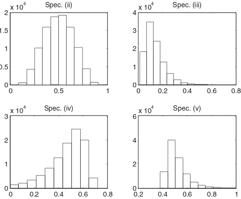
We consider five different specifications for the instrument propensity score function: (i) Constant:q(X)=0.6; (ii) Linear 1:q(X)=(−2.5+g(X)); (iii) Linear 2: q(X)=(−4.5+
g(X)); (iv) Rational expression 1: q(X)=(2−5/g(X)); (v) Rational expression 2:q(X)=(−1+2.5/g(X)). The dis-tribution of the random variableq(X) in the various cases is shown inFigure 1.
The constant specification (i) represents the benchmark case in which the instrument is completely randomly assigned; it will also serve as an illustration of how covariates thatq(·) does not depend on can still be used in estimation to improve efficiency. The linear specifications (ii) and (iii) are functions that are easily estimable by SLE; in fact, here SLE acts as a correctly specified or overspecified parametric estimator. Model (iii) will also pose a challenge to the asymptotic results asq(X) concentrates a lot of mass close to zero. Finally, the rational models (iv) and (v) are intended to be true “nonparametric” specifications in that any implementation of the SLE based on a fixed number of powers is, in theory, only an approximation to the true function (though a quadratic approximation seems already adequate in practice). Of the two, specification (v) stays safely away from
0 0.5 1
0 0.5 1 1.5
2x 10
4 Spec. (ii)
0 0.2 0.4 0.6 0.8
0 1 2 3 4x 10
4 Spec. (iii)
0 0.2 0.4 0.6 0.8
0 1 2 3x 10
4 Spec. (iv)
0.2 0.4 0.6 0.8 1
0 2 4 6x 10
4 Spec. (v)
Figure 1. The distribution ofq(X).
zero and one, while (iv) puts a fair amount of weight in a close neighborhood of zero.
Clearly, the DGP satisfies one-sided noncompliance as
D(0)=0. The value of the parameter b∈[0,1] governs whether the unconfoundedness assumption is satisfied. In par-ticular, when b=0 unconfoundedness holds conditional on
X2=X. Larger values of b correspond to more severe
vio-lations of the unconfoundedness assumption. The instrumentZ is valid conditional onX1=Xfor anyb.
To make a credible case for unconfoundedness in practice, one often needs a large number of theoretically relevant co-variates. Here we use five, which is likely insufficient in a lot of applications. Nevertheless,Xis large enough to allow us to make a number of salient points without posing an undue com-putational burden. In Section6, we will present an additional, smaller Monte Carlo exercise where the setup is based on a real dataset with up to 14 covariates.
5.1 The Finite Sample Distribution of the LATE Estimator
In our first exercise, we study the finite sample distribution of the LATE estimator ˆτ. The DGP is designed so that the true value of the LATE parameter is independent ofq(·) and is approximately equal toτ = −2.73 forb=0.5, the value chosen for this exercise.
Table C.1 shows various statistics characterizing the finite sample distribution of ˆτ and its estimated standard error for
n=250,n=500,andn=2500. In particular, we report the bias of ˆτ, the standard error ofT ≡√n( ˆτ −τ), the mean es-timate of this standard error based on comment 3 after The-orem 1, and the tail probabilities of the studentized estimator
S≡( ˆτ−Eτˆ)/s.e.( ˆτ) associated with the critical values−1.645 and 1.645. The number of Monte Carlo repetitions is 5000.
For each specification ofq(·), we consider a number of im-plementations of the SLE. We start with a constant model for the instrument propensity score and then add linear, quadratic, and cubic terms (all powers of Wi and all cross products up
to the given order). We use the same power series to estimate all other nonparametric components of the influence function (used in estimating the standard error of ˆτ). The choice of the power series in implementing the SLE is an important one; it mimics the choice of the smoothing parameter in kernel-based or local polynomial estimation. To our knowledge, there is no well-developed theory to guide the power series choice in finite samples (though Imbens, Newey, and Ridder2007is a step in this direction); hence, a reasonable strategy in practice would involve examining the sensitivity of results to various specifica-tions as is done in this simulation.
When using an IPW estimator in practice, the estimated prob-abilities are often trimmed to prevent them from getting too close to, the boundaries of the [0,1] interval. Therefore, we also ap-ply trimming to the raw estimates delivered by the SLE. The column “Trim.” inTable C.1denotes the truncation applied to the estimated instrument propensity scores. If the fitted value
ˆ
q(Xi) is strictly less than the threshold γ ∈(0,1/2), we reset
ˆ
q(Xi) toγ. Similarly, if ˆq(Xi) is strictly greater than 1−γ, we
reset ˆq(Xi) to 1−γ. We useγ =0.5% (mild trimming) and,
occasionally,γ =5% (aggressive trimming). The latter is only
applied to specifications (ii=Linear 2) and (iv=Rational 1), where the boundary problem is the most severe.
Many aspects of the results displayed in Table C.1 merit discussion.
First, looking at the simplest case when neitherqnor ˆq de-pends onX, we see that even forn=250, the bias of the LATE estimator is very small, its estimated standard error, too, is prac-tically unbiased, and the distribution of the studentized estimator has tail probabilities close to standard normal. Even though the true instrument propensity score does not depend on the co-variates, one can achieve a substantial reduction in the standard error of the estimator by allowing ˆqto be a function ofX, as sug-gested by Theorem 3 of Fr¨olich and Melly (2013b). For example, when ˆq(X) is linear, the standard error, forn=2500, falls from about 3.21 to 2.42, roughly a 25% reduction. Nevertheless, we can also observe that if ˆq(X) is very generously parameterized (here: quadratic), then in small samples the “noise” from esti-mating too many zeros can overpower most of this efficiency gain. Specifically, forn=250 the standard error of the scaled estimator is almost back up to the noncovariate case (3.16 vs. 3.23). Still, the efficiency gains are recaptured for largen.
A second, perhaps a bit more subtle, point can be made about the standard error of ˆτusing the Linear 1 specification forq(X). Here, the linear SLE acts as a correctly specified parametric es-timator while the estimated standard errors are computed under the assumption that q is nonparametrically estimated. Thefore, the estimated standard errors are downward-biased, re-flecting the fact that even when the instrument propensity score is known up to a finite-dimensional parameter vector, it is more efficient to use a nonparametric estimator in constructing ˆτ as in Chen, Hong, and Tarozzi (2008). Indeed, as the SLE adds quadratic and cubic terms, that is, it starts “acting” more as a nonparametric estimator, the bias vanishes from the estimated standard errors, provided that the sample size expands simulta-neously (n=2500). Furthermore, the asymptotic standard er-rors associated with the quadratic and cubic SLE (2.72 and 2.93, respectively) are lower than for the linear (3.11). In cases where the variance of ˆτ is underestimated, the studentized estimator tends to have more mass in its tails than the standard normal distribution (see, e.g., the results for the linear SLE).
Third, as best demonstrated by the Linear 2 model for the instrument propensity score, the limit distribution provided in Theorem 1 can be a poor finite sample approximation when
q(X) gets close to zero or one with relatively high probability. This is especially true when the estimator forq(X) is overspec-ified (quadratic or cubic). Forn=250 andn=500, the bias of
ˆ
τ ranges from moderate to severe and is exacerbated by more aggressive trimming of ˆq. For any series choice, the standard error of the LATE estimator is larger than in the Linear 1 case (the 0.5% vs. 5% trimming does not change the actual standard errors all that much). Furthermore, for ˆqquadratic or cubic, the estimated standard errors are severely upward biased with mild trimming, and still very much biased, though in the opposite direction, with aggressive trimming. Increasing the sample size ton=2500 of course lessens these problems, though judging from the tail probabilities, the standard normal can remain a rather crude approximation to the studentized estimator. For ex-ample, for the cubic SLE with 0.5% trimming the standard error is grossly overestimated and there is evidence of skewness. On
the other hand, for the linear and quadratic SLE the estimated asymptotic standard errors display downward bias, presumably due to the “correct parametric specification” issue discussed in the second point above. Somewhat surprisingly, though, the actual standard errors are the smallest for the linear SLE; appar-ently, even forn=2500, there is more than “optimal” noise in the quadratic and cubic instrument propensity score estimates.
Fourth, when the instrument propensity score estimator is un-derspecified, ˆτ is an asymptotically biased estimator of LATE. (Here “underspecified” refers to a misspecified model in the parametric sense or, in the context of series estimation, extend-ing the power series too slowly as the sample size increases.) The bias is well seen in all cases in which the instrument propensity score depends onX, but is estimated by a constant. The Rational 1 and Rational 2 models provide further illustration. Here, any fixed power series implementation of the SLE is misspecified if regarded as a parametric model, though the estimator pro-vides an increasingly better approximation toq(·) as the power series expands. For the Rational 1 model, the bias of ˆτ indeed decreases in magnitude as the SLE becomes more and more flexible, with the exception ofn=250. For Rational 2, even the linear SLE removes the bias almost completely and not much is gained, even asymptotically, by using a more flexible estimator. For Rational 1, there is noticeable asymptotic bias in estimat-ing the standard error of ˆτ, which would presumably disappear if the sample size and the power series both expanded further. Nevertheless, for both rational models the normal approxima-tion to ˆτ works reasonably well in large samples across a range of implementations of the SLE.
Finally, the results as a whole show the sensitivity of ˆτ to the specification of the power series used in estimating the in-strument propensity scoreq(·). If the power series has too few terms (or expands too slowly with the sample size), then ˆτ may be (asymptotically) biased. On the other hand, using too flexible a specification for a given sample size can cause ˆτto have severe small sample bias and inflated variance, which is also estimated with bias. More aggressive trimming of the instrument propen-sity score tends to increase the bias of ˆτ and reduce the bias of
s.e.( ˆτ), though to an uncertain degree.
5.2 Properties of the Test and the Pretested Estimator
We first set b=0 so that unconfoundedness holds for any specification of q(X) conditional on X2=X. All tests are
conducted at the 5% nominal significance level and with
X1=X2=X, that is, we drop the cases where ˆq is constant.
To further economize on space, we also drop the 5% truncation for the Rational 1 specification. In each of the remaining cases, we consider four estimators of (L)ATT: ˆτt, ˆβt, their combination
ˆ
βt( ˆa), and a pretested estimator, given by ˆβt( ˆa) whenever the test
accepts unconfoundedness and ˆτt when it rejects it. Trimming
is also applied to ˆp(·).
In Tables C.C.2and C.C.3, we report, for each estimator, the raw bias, the standard deviation of√n((L)ATT −(L)ATT), the mean of the estimated standard deviation, and the mean squared error of√n((L)ATT −(L)ATT). We use a naive (but natural) es-timator for the standard error of the pretested eses-timator; namely, we take the estimated standard error of either ˆβt(a) or τt,
de-pending on which one is used. In addition, we report the actual rejection rates and the average weight across Monte Carlo cycles that the combined estimator assigns to ˆτt(the mean of ˆa).
Again, several aspects of the results are worth discussing. First, there is adequate, though not perfect, asymptotic size control in all cases, where the specification of the SLE is suffi-ciently flexible and there is no excessive trimming. The extent to which the 5% trimming can distort the size of the test in the Linear 2 case is rather alarming; in the very least, this suggests that trimming should be gradually eliminated as the sample size increases.
Second, in almost all cases, the combined estimator has smaller standard errors in small samples than the HIR estimator
ˆ
βt, and the drop is especially large when ˆq is overspecified.
While this tends to be accompanied by an uptick in absolute bias, in almost all cases the combined estimator has the lowest finite sample MSE—the only exceptions come from the Linear 2 model with aggressive trimming. As the DGP satisfies the conditions of Theorem 3, the combined estimator puts less and less weight on ˆτt in larger samples and becomes equivalent to
ˆ
βtunless trimming interferes.
Third, even though the pretested estimator has a higher MSE than ˆβt or the combined estimator, in almost all the cases this
MSE is lower than that of ˆτt. (Again, the only exceptions come
in the Linear 2 case with 5% trimming forn=2500, but here ˆ
βt itself has a higher MSE than ˆτt.) Thus, while there is a
price to pay for testing the validity of the unconfoundedness assumption, there is still a substantial gain relative to the case where one only has the IV estimator to fall back on. Of course, one would be better off taking unconfoundedness at face value when it actually holds. But as we will shortly see, there is a large cost in terms of bias if one happens to be wrong, and the consistency of the unconfoundedness test helps avoid paying this cost.
Fourth, the naive method described above underestimates the true standard error of the pretested estimator. We briefly exam-ined a bootstrap estimator in a limited number of cases, and the results (not reported) appear upward biased. We do not con-sider these results conclusive as we took some shortcuts due to computational cost (to study this estimator one has to embed a bootstrap cycle inside a Monte Carlo cycle). We further note that the distribution of the pretested estimator can show severe departures from normality such as multimodality or extremely high kurtosis.
We now present cases where unconfoundedness does not hold conditional onX. Specifically, we setb=0.5 again; some addi-tional results forb=0.25 are available in an online supplement. We focus only on those cases from the previous exercise where size was asymptotically controlled, as power has questionable value otherwise. The results are displayed in Table C.4.
Our first point is that the test appears consistent against these departures from the null—rejection rates approach unity as the sample size grows in all cases examined. Nevertheless, over-specifying the series estimators can seriously erode power in small samples; see the cubic SLE in Table C.4 forq=Linear 1, Rational 1, Rational 2. In fact, in these cases the test is not unbiased. A further odd consequence of overfitting is that power need not increase monotonically withn; see again the cubic SLE in Table C.4 forq=Linear 2.
Second, ˆβt, and hence the combined estimator, is rather
severely biased both in small samples and asymptotically (the bias is of course a decreasing function ofb). Therefore, even though ˆβtgenerally has a lower standard error than ˆτt, its MSE,
in large enough samples, is substantially larger than that of ˆτt. As
the sample size grows, the pretested estimator behaves more and more similarly to ˆτt, eventually also dominating ˆβt and ˆβt( ˆa).
Third, in smaller samples the MSE of the pretested estimator is often larger than that ofτtas the pretested estimator uses ˆβt( ˆa)
with positive probability, and ˆβt( ˆa) is usually inferior to ˆτt due
to its bias inherited mostly from ˆβt. However, there are cases in
which the increased bias of the combined estimator is more than offset by a reduction in variance so that MSE( ˆβt( ˆa)) is lower
than MSE( ˆτt) or MSE( ˆβt) or both. This happens mainly when
n=250 and ˆq is overspecified; see also the cubic SLE forq= Linear 1, Linear 2, Rational 1, Rational 2 in Table C.4. As in these cases power tends to be (very) low, the pretested estimator preserves most of the MSE gain delivered by ˆβt( ˆa) or might even
improve on it slightly. This property of the combined estimator mitigates the cost of the Type 2 errors made by the test.
6. EVALUATING THE UNCONFOUNDEDNESS TEST USING REAL DATA
6.1 An Illustrative Empirical Application
We apply our method to estimate the impact of JTPA training programs on subsequent earnings and to test the unconfoundedness of the participation decision. We use the same dataset as Abadie, Angrist, and Imbens (2002), hence-forth AAI, publicly available at http://econ-www.mit.edu/ faculty/angrist/data1/data/abangim02. As described by Bloom et al. (1997) and AAI, part of the JPTA program (the National JTPA study) involved collecting data specifically for purposes of evaluation. In some of the service delivery areas, between November 1987 and September 1989, randomly selected ap-plicants were offered a job-related service (classroom training, on-the-job training, job search assistance, etc.) or were denied services and excluded from the program for 18 months (1 out of 3 on average).
Clearly, the random offer of services (Z) can be used, without further conditioning, as an instrument for evaluating the effect of actual program participation (D) on earnings (Y), measured as the sum of earnings in the 30-month period following the offer. About 36% of those with an offer chose not to participate; conversely, a small fraction of applicants, less than 0.5%, ended up participating despite the fact that they were turned away. Hence,Z satisfies one-sided noncompliance almost perfectly; the small number of observations violating this condition were dropped from the sample. (AAI also ignores this small group in interpreting their results.) The total number of observations is then 11,150; of these, 6067 are females and 5083 are males. We treat the two genders separately throughout.
The full set of AAI covariates (X) include
“dummies for black and Hispanic applicants, a dummy for high-school graduates (including GED holders), dummies for married applicants, 5 age-group dummies, and dummies for AFDC receipt (for women) and whether the applicant worked at least 12 weeks in the 12 months preceding random assignment. Also included are dummies for the original recommended service strategy [. . .] and a dummy for whether earnings data are from the second follow-up survey.” (AAI, p. 101)
SeeTable 1of AAI for descriptive statistics. To illustrate the “sample splitting” method described in Comment 6 after Theo-rem 1 we also construct a smaller set of controls with dummies for high-school education, minority status (black or hispanic), and whether the applicant is below age 30 years.
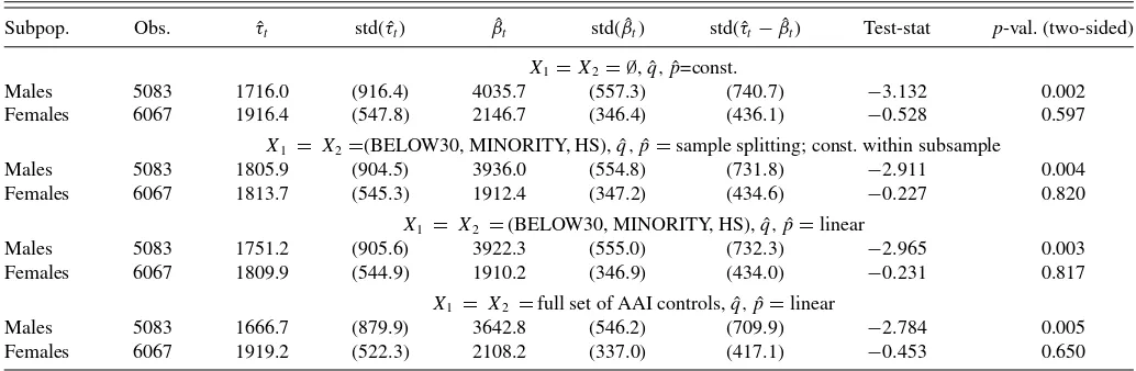
InTable 1, we present four sets of estimation/test results. In the first exercise, we do not use any covariates in computing ˆτt
and ˆβt. The LATT estimator ˆτt is interpreted as follows. Take,
for example, the value 1916.4 for females. This means that female compliers who actually participated in the program (i.e., were assignedZ=1), are estimated to increase their 30-month earnings by $1916.4 on average. SinceZis randomly assigned, this number can also be interpreted as an estimate of LATE, that is, the average effect among all compliers. Further, by one-sided noncompliance, $1916.4 is also an estimate of the female ATT. As the difference between ˆτtand ˆβt=2146.7 is not statistically
significant, the hypothesis of completely randomparticipation cannot be rejected for females. In contrast, ˆβtfor males is more
Table 1. Treatment effect estimates and unconfoundedness test results
Subpop. Obs. τˆt std( ˆτt) βˆt std( ˆβt) std( ˆτt−βˆt) Test-stat p-val. (two-sided)
X1=X2= ∅, ˆq,pˆ=const.
Males 5083 1716.0 (916.4) 4035.7 (557.3) (740.7) −3.132 0.002 Females 6067 1916.4 (547.8) 2146.7 (346.4) (436.1) −0.528 0.597
X1 = X2=(BELOW30, MINORITY, HS), ˆq,pˆ=sample splitting; const. within subsample
Males 5083 1805.9 (904.5) 3936.0 (554.8) (731.8) −2.911 0.004 Females 6067 1813.7 (545.3) 1912.4 (347.2) (434.6) −0.227 0.820
X1 = X2 =(BELOW30, MINORITY, HS), ˆq,pˆ=linear
Males 5083 1751.2 (905.6) 3922.3 (555.0) (732.3) −2.965 0.003 Females 6067 1809.9 (544.9) 1910.2 (346.9) (434.0) −0.231 0.817
X1 = X2 =full set of AAI controls, ˆq,pˆ=linear
Males 5083 1666.7 (879.9) 3642.8 (546.2) (709.9) −2.784 0.005 Females 6067 1919.2 (522.3) 2108.2 (337.0) (417.1) −0.453 0.650
Note:τˆtis the IPW IV estimator of (L)ATT. ˆβtis the IPW estimator of ATT under unconfoundedness. All estimates are in U.S. dollars (ca. 1990). Numbers in parentheses are standard
errors.
than twice as large as ˆτt, and the difference is highly significant.
This suggests that self-selection into the program among men is based partly on factors systematically related to the potential outcomes.
In the next two exercises, we set X1 and X2 equal to the
restricted set of covariates. First, we split the male and female samples by the eight possible configurations of the three in-dicators and estimate the instrument propensity score by the subsample averages ofZ; then we restrict the functional form to logit with a linear index. The two sets of results are similar both to each other and the results from the previous exercise. In particular, random participation is not rejected for females, while it is still strongly rejected for males. There are factors related to the male participation decision as well as the potential outcomes that are not captured by the set of covariates used.
Finally, in the fourth exercise we use the full set of AAI co-variates in a linear logit model. Compared with the no-covariate case, the estimated standard errors are slightly lower across the board, but the changes in the point estimates are still within a small fraction of them. Once again, the test does not reject uncounfoundedness for females but it does for males.
Since the hypothesis of random treatment participation can-not be rejected for females, ˆβt can also be interpreted as an
estimate of ATE. In contrast, ˆβt is likely to be substantially
bi-ased as an estimate of male ATE. Furthermore, bbi-ased on Section 4, one can take a weighted average of ˆτtand ˆβtto obtain a more
efficient estimate of female ATE/ATT. As ˆa≈0 in all cases, the combined estimator is virtually the same as ˆβt and is not
reported. Nevertheless, without testing for (and failing to re-ject) the unconfoundedness assumption, the only valid estimate of female ATT is ˆτt, which has a much larger standard error
than ˆβt.
While the result on male versus female self-selection is ro-bust in this limited set of exercises, one would need to study the program design in more detail before jumping to conclusions about, say, behavioral differences. Understanding how the ex-plicitly observed violations of one-sided noncompliance came about would be especially pertinent, and, as pointed out by a referee, the broader issue of control group substitution docu-mented by Heckman, Hohmann, Smith, and Khoo (2000) would also have to be taken into account. Furthermore, there are poten-tially relevant covariates (e.g., indicators of the service delivery area) not available in the AAI version of the dataset. In short, the empirical results are best treated as illustrative or as a starting point for a more careful investigation.
6.2 An Empirical Monte Carlo Exercise
We supplement our illustrative application with an empirical Monte Carlo exercise. The basic idea, as described by Huber et al. (2013), is to build a data-generating process in which the number of variables, their distributions, and the relationships between them are based on empirical quantities from a rele-vant dataset (the AAI version of the JTPA data in our case). Of course, in evaluating our test procedure we need to control whether or not the null hypothesis holds, which makes it neces-sary to introduce some artificial variables and parameters. We focus the exercise on a question left unexplored in our “syn-thetic” Monte Carlo study; namely, the potential distortions
introduced by violations of the one-sided noncompliance as-sumption. The simulations also provide additional evidence on the size and power properties of the test in a presumably more realistic setting. Similarly to the application, we condition on gender throughout, that is, treat males and females as separate populations.
Mimicking the experimental setup in the National JTPA study, the instrumentZis a random draw from a Bernoulli(2/3) distri-bution. Let ˆθdenote the coefficient vector from a logit regression of the observed treatment indicator on a constant and the full set Xof the AAI covariates. The potential treatment status indicator
D(1) is generated according to
D(1)=1((X′θˆ+bν)> U),
where(·) is the logistic cdf,U∼uniform[0,1],ν∼N(0,1), independent of each other,XandZ. The parameterb≥0 gov-erns how strong a role the unobserved variableν plays in the selection process;D(0) and the potential outcomes will be spec-ified in a way so that unconfoundedness holds if and only if
b=0, that is,νis the only unobserved confounder. We define
D(0) in two different ways:
(i)D(0)=D(1)·1((ν)< c) and (ii)D(0)=D(1)·1(S < c),
where(·) is the standard normal cdf,S is uniform[0,1], in-dependent of all other variables defined thus far, andc∈[0,1] is a parameter that we calibrate to setπ ≡P[D(0)=1] equal to various prespecified values. (For example, forc=0,π =0 for both specifications.) The multiplicative structure ofD(0) en-sures that monotonicity is satisfied, that is, there are no defiers in the population. In specification (i) the violation of one-sided noncompliance is due to the confounding variableν; in case (ii) it is due to a completely exogenous variable. Actual treatment status isD=D(Z).
The potential outcomeY(1) is drawn randomly from the em-pirical distribution of earnings (regardless of treatment status in the data), andY(0) is specified as
Y(0)=Y(1)−0.2 ˆσ(α+X′θˆ+ν+ǫ),
where ǫ∼N(0,1) is an independently generated error, ˆσ is the standard deviation of earnings in the data, andα= −0.47 for males and−0.06 for females. The potential outcome equa-tions were calibrated so that for b=1 and π =0, ATT= LATT≈1667 in the male population, and forb=0 andπ=0, ATT=LATT≈1920 in the female population. These settings match the value of ˆτt in the last panel of Table 1as well as
the conclusion of the test in the two populations. The actually observed outcome is of courseY =Y(D).
In each Monte Carlo cycle, we draw a sample of sizenM
for males and nF for females. We perform the
unconfound-edness test at the 5% nominal significance level, using the specifications given in the bottom panel ofTable 1. The cho-sen sample sizes arenF =500; 5000 andnM =600; 6000 (the
larger figure for either gender matches the application). We report rejection rates for various values of the parameters b and π =P[D(0)=1]. For females, we restrict attention to the size of the test (b=0), while for males we study size as well as power (b=0,0.5,0.75,1,1.25). We calibratecto give
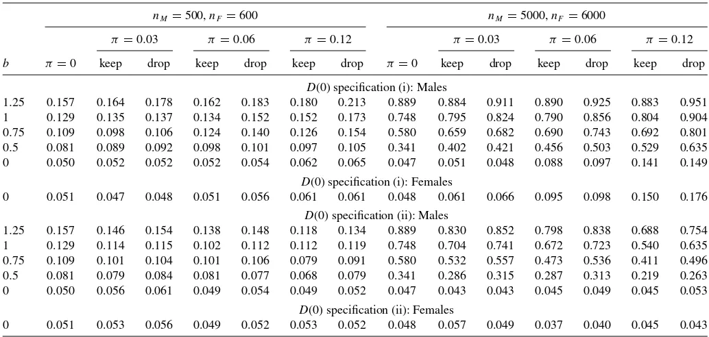
Table 2. Empirical Monte Carlo: rejection rates of the unconfoundedness test at the 5% nominal significance level
nM=500,nF =600 nM=5000,nF=6000
π=0.03 π =0.06 π=0.12 π =0.03 π=0.06 π=0.12
b π=0 keep drop keep drop keep drop π=0 keep drop keep drop keep drop
D(0) specification (i): Males
1.25 0.157 0.164 0.178 0.162 0.183 0.180 0.213 0.889 0.884 0.911 0.890 0.925 0.883 0.951 1 0.129 0.135 0.137 0.134 0.152 0.152 0.173 0.748 0.795 0.824 0.790 0.856 0.804 0.904 0.75 0.109 0.098 0.106 0.124 0.140 0.126 0.154 0.580 0.659 0.682 0.690 0.743 0.692 0.801 0.5 0.081 0.089 0.092 0.098 0.101 0.097 0.105 0.341 0.402 0.421 0.456 0.503 0.529 0.635 0 0.050 0.052 0.052 0.052 0.054 0.062 0.065 0.047 0.051 0.048 0.088 0.097 0.141 0.149
D(0) specification (i): Females
0 0.051 0.047 0.048 0.051 0.056 0.061 0.061 0.048 0.061 0.066 0.095 0.098 0.150 0.176
D(0) specification (ii): Males
1.25 0.157 0.146 0.154 0.138 0.148 0.118 0.134 0.889 0.830 0.852 0.798 0.838 0.688 0.754 1 0.129 0.114 0.115 0.102 0.112 0.112 0.119 0.748 0.704 0.741 0.672 0.723 0.540 0.635 0.75 0.109 0.101 0.104 0.101 0.106 0.079 0.091 0.580 0.532 0.557 0.473 0.536 0.411 0.496 0.5 0.081 0.079 0.084 0.081 0.077 0.068 0.079 0.341 0.286 0.315 0.287 0.313 0.219 0.263 0 0.050 0.056 0.061 0.049 0.054 0.049 0.052 0.047 0.043 0.043 0.045 0.049 0.045 0.053
D(0) specification (ii): Females
0 0.051 0.053 0.056 0.049 0.052 0.053 0.052 0.048 0.057 0.049 0.037 0.040 0.045 0.043
Note:Forπ=0 one-sided noncompliance is satisfied and specifications (i) and (ii) coincide.
π=0,0.03,0.06, and 0.12, where π=0 implies that one-sided noncompliance is satisfied. Whenπ >0, we perform the test in two different ways: first we keep individuals that appar-ently violate one-sided noncompliance (“keep”) and then we drop them from the sample (“drop”); the expected proportion of such observations isπ/3. The number of Monte Carlo repeti-tions is 2500 for the smaller values ofnM andnF, and 1000 for
the larger.
The simulation results are presented in Table 2. Under specification (i), violation of one-sided noncompliance causes ATT=LATT. Theory predicts that in this case our test statistic explodes, even forb=0, asn→ ∞. Viewed as a test of the unconfoundedness assumption, this amounts to potentially se-vere size distortion, while the effect on finite sample power is generally ambiguous (the bias in ˆβtwhenb=0 might partially
offset the difference between ATT and LATT or add to it). As shown by panel (i) inTable 2, there is little evidence of size distortion fornM =500 andnF =600, even whenπ=0.12.
However, power is also quite poor, likely because the number of covariates used in estimating the propensity score is fairly large relative to the sample size (dim(X)=13 for males and 14 for females). This observation accords well with the earlier find-ing in the traditional Monte Carlo exercise that overspecifyfind-ing the propensity score estimator can lead to severe reduction in power. FornM =5000 andnF =6000, size distortion becomes
quite significant. Forπ=0.06, actual size is roughly double the nominal size for either gender, while forπ =0.12 it is triple. At the same time, power also increases significantly, and it is interesting to note that even after adjusting for the size distor-tion, power tends to be larger forπ >0 than forπ =0, at least for smaller positive values ofband the “drop” option.
Specification (ii) forD(0) represents a polar case in which one-sided noncompliance is violated, but the significance level of the test is unaffected, because ATT=LATT. This is a
con-sequence of the fact thatZ is completely randomly assigned, andD(0) is completely randomly assigned whenD(1)=1. It is straightforward to show that in this case the common value of the two parameters is given byE[Y(1)−Y(0)|D(1)=1]. Indeed, as shown by panel (ii) ofTable 2, the nominal 5% size remains valid even for nM =5000 andnF =6000. There is
however evidence that violation of one-sided noncompliance reduces power, suggesting that the bias of ˆβt is a (slightly)
de-creasing function ofπfor a givenb >0. Also, the “drop” option seems to result in a small upward shift in the entire finite sample power curve.
Generally speaking, the results suggest that the rejection of the unconfoundedness assumption for males in the empirical exercise is unlikely to be a product of potential size distortions caused by the apparently mild violation of one-sided noncom-pliance (in the applicationP[D(0)=1]≈3×0.005=0.015). On the other hand, the nonrejection for females could reflect lack of power against moderate violations of unconfounded-ness. In the setup considered above, the unobserved confounder
ν must play a significant role in the selection process for un-confoundedness to be rejected with reasonably high probability. For example, for males var(bν)/var(X′θˆ)≈1.5 forb=0.5, and still power is only about 34% forπ =0 andnM =5000.
7. CONCLUSION
Given a (conditionally) valid binary instrument, nonparamet-ric estimators of LATE and LATT can be based on imputation or matching, as in Fr¨olich (2007), or weighting by the estimated instrument propensity score, as proposed in this article. The two approaches are shown to be asymptotically equivalent; in par-ticular, both types of estimators are√n-consistent and efficient. When the available binary instrument satisfies one-sided non-compliance, the proposed estimator of LATT is compared with