INTEGRATED RENEWAL PROCESS

(1)

Suyono and J.A.M. van der Weide

Abstract. The marginal distribution of integrated renewal process is derived in this paper. Our approach is based on the theory of point processes, especially Poisson point processes. The results are presented in the form of Laplace transforms.

1. INTRODUCTION

Consider arrival of passengers at a train station and model this situation as a re-newal process. It means that the inter-arrival times between consecutive passengers are assumed to be independent and identically distributed (iid) non-negative ran-dom variables. Suppose that at a certain time (time 0) a train is just departed from the station and there are no passengers left. Passengers who come after the time 0 have to wait until the departure of the next train at some time pointt≥0. We are interested in the waiting time of these passengers. The total waiting time of all passengers in the time interval [0,t] is an example of a stochastic process which we call an integrated renewal process. The nomenclature becomes clear from the mathematical definition of the process in Section 2.

An integrated renewal process can be considered as a generalization of a stochastic process which we call an integrated Poisson process in this paper. The expected value of the integrated Poisson process has been discussed in Ross [6]. The integrated renewal process has also a close connection with shot noise processes discussed by Gubner [4]. For asymptotic properties of this process, see Suyono and Van der Weide (2007). In this paper we discuss the marginal distribution of this process which is important for analyzing probabilistic characterizations of the process at any time point.

This paper is organized as follows. In Section 2 we give a mathematical definition of an integrated renewal process. In Section 3 we consider an integrated

Received 8 November 2006, revised 4 January 2007, accepted 15 November 2007. 2000 Mathematics Subject Classification: 60K05

Key words and Phrases: renewal process, point process, Laplace transform

(2)

Poisson process including the variance and the marginal probability density function of the process. In Section 4 we consider the marginal distribution of integrated renewal process and in the last section we give an example.

2. DEFINITIONS

Let (Xn, n ≥ 1) be an iid sequence of non-negative random variables having a

common distribution functionF. LetSn =Pni=1Xi, n≥1, and set S0= 0. The process (N(t), t≥0) where

N(t) = sup{n≥0 :Sn≤t}

is known as a renewal process. In the sequel we will interpret the variablesXn as

inter-arrival times of the renewal process. Define fort≥0

Y(t) = Z t

0

N(s)ds.

We call the stochastic process (Y(t), t≥0)integrated renewal process. As a special case, if (N(t), t ≥ 0) is a Poisson process then we call the process (Y(t), t ≥ 0)

integrated Poisson process. Note that we can expressY(t) as

Y(t) =

N(t) X

i=1

(t−Si) =tN(t)−Z(t), (1)

where

Z(t) =

N(t) X

i=1

Si. (2)

So if we interpretSn,n= 1,2,3, ...as arrival times of passengers in a train station

thenY(t) represents the total waiting time of all passengers until the departure of a train at timet. In the next sections we will discuss the marginal distributions of Y(t) andZ(t).

3. INTEGRATED POISSON PROCESS

Firstly, suppose that the process (N(t), t≥0) is an homogeneous Poisson process with rateλ >0. It is well known that givenN(t) =n, thenarrival timesS1, ..., Sn

have the same distribution as the order statistics corresponding ton independent random variables uniformly distributed on the time interval [0, t], see e.g. Ross [6]. Conditioning on the number of arrivals in the time interval [0, t] we obtain

E(e−αY(t)₎ ₌

∞

X

n=0

Ehe−αPn

i=1(t−Si)_|_N_{(t) =}_n

i

(3)

=

where Ui, i= 1,2, ..., nare independent and identically uniform random variables

on [0, t]. Since

it follows that

E(e−αY(t)_{) = exp} argument we can prove thatZ(t) has the same Laplace transform asY(t). So by uniqueness theorem for Laplace transforms we conclude that for each t, Y(t) and Z(t) have the same distribution.

The distribution ofY(t) has a mass at zero with P(Y(t) = 0) = e−λt_. _The

probability density function fY(t) of the continuous part of Y(t) can be obtained by inverting the Laplace transform in (3). Note that we can express (3) as

E(e−αY(t)₎ ₌ _e−λt

Inverting this transform we obtain, forx >0,

fY(t)(x)

whereIk(x) is the Modified Bessel function of the first kind, i.e.,

Ik(x) = (1/2x)k

(4)

For large t, the distribution of Y(t) can be approximated by the normal distribution having mean 1₂λt2 _{and variance} 1

3λt3. To prove this we will consider the characteristic function of the normalized Y(t). Firstly, note that

E

−1 and an expansion we obtain

E

which is the characteristic function of the standard normal distribution.

Now consider the case where (N(t)) is a non-homogeneous Poisson process with intensity measureν. GivenN(t) =n, the arrival times Si, i= 1,2, ..., nhave

the same distribution as the order statistics of n iid random variables having a common cumulative distribution function

G(x) = (

ν([0,x])

ν([0,t]), x≤t 1, x > t.

By conditioning on the number of arrivals in the time interval [0, t] we get

E³e−αZ(t)´ _{= exp}

From this Laplace transform we deduce that

E[Z(t)] =

Similarly, we can prove that

E(e−αY(t)_{) = exp}

(5)

4. INTEGRATED RENEWAL PROCESS

In this section we will consider the marginal distributions of the processes (Y(t)) and (Z(t)) defined in (1) and (2) for the case that (N(t)) is a renewal process. We will assume that the inter-arrival times Xn of the renewal process (N(t)) are

strictly positive. First we consider the process (Z(t)). Obviously we can express Z(t) as

Z(t) =

N(t) X

i=1

[N(t) + 1−i]Xi. (4)

We will use point processes to derive the marginal distribution ofZ(t).

Let (Ω,F,P) be the probability space on which the iid sequence (Xn) is

defined and also an iid sequence (Vn, n≥1) of exponentially distributed random

variables with parameter 1 such that the sequences (Xn) and (Vn) are independent.

Let (Tn, n≥1) be the sequence of partial sums of the variablesVn. Then the map

Φ : ω 7→ P∞

n=1δ(Tn(ω),Xn(ω)), (5)

where δ(x,y) is the Dirac measure in (x, y), defines a Poisson point process on E= [0,∞)×[0,∞) with intensity measureν(dtdx) =dtdF(x), see Resnick [5]. Let Mp(E) be the set of all point measures onE. We will denote the distribution of Φ

byPν, i.e.,Pν =P◦Φ−1.

Define fort≥0 the functionalA(t) onMp(E) by

A(t)(µ) = Z

E

1[0,t)(s)xµ(dsdx). (6)

In the sequel we write A(t, µ) =A(t)(µ). Suppose that the point measure µ has the support supp(µ) = ((tn, xn))∞n=1 witht1< t2< . . .. It follows that

µ=

∞

X

n=1 δ(tn,xn)

andA(t, µ) can be expressed as

A(t, µ) =

∞

X

n=1

1[0,t)(tn)xn.

Note that for everyt≥0,A(t, µ) is almost surely finite. Define also fort≥0 the functionalZ(t) onMp(E) by

Z(t)(µ) = Z

E

Z

E

1[0,x)(t−A(s, µ))µ([r, s)×[0,∞))u1[0,s)(r)µ(drdu)µ(dsdx).

(6)

Lemma 4.1. With probability 1,

Z(t) =Z(t)(Φ).

Proof. Letω∈Ω. Then

Z(t)(Φ(ω))

=

∞

X

n=1

1[0,Xn(ω))(t−A(Tn(ω),Φ(ω)))

∞

X

i=1

Φ(ω)([Ti(ω), Tn(ω))×[0,∞))Xi(ω)1[0,Tn(ω))(Ti(ω))

=

∞

X

i=1

Φ(ω)([Ti(ω), TN(t,ω)+1(ω))×[0,∞))Xi(ω)1[0,TN(t,ω)+1(ω))(Ti(ω))

=

N(t,ω) X

i=1

[N(t, ω) + 1−i]Xi(ω). ¤

Theorem 4.1. Let (Xn, n ≥ 1) be an iid sequence of strictly positive random variables with common distribution function F. Let (Sn, n ≥ 0) be the sequence of partial sums of the variables Xn and(N(t), t≥0) be the corresponding renewal process: N(t) = sup{n≥0 :Sn ≤t}. Let

Z(t) =

N(t) X

i=1

[N(t) + 1−i]Xi.

Then for α, β >0

Z ∞

0

E(e−αZ(t)_)e−βt_dt₌ 1

β[1−F

∗_(β_)]

∞

X

n=0

n

Y

i=1

F∗_(α[n_{+ 1}₋_{i] +}_β) ₍₇₎

(with the usual convention that the empty product equals 1), whereF∗ _{denotes the}

Laplace-Stieltjes transforms of F. Proof. By Lemma 4.1.

E(e−αZ(t)₎

= Z

Mp(E)

e−αZ(t)(µ)_P

ν(dµ)

= Z

Mp(E)

exp ½

−α Z

E

Z

E

1[0,x)(t−A(s, µ))

µ([r, s)×[0,∞))u1[0,s)(r)µ(drdu)µ(dsdx) ¾

(7)

=

Applying the Palm formula for Poisson point processes, see Grandell [3], we obtain

E(e−αZ(t)₎

Using Fubini’s theorem and a substitution we obtain

Z ∞

The integral with respect to Pν can be written as a sum of integrals over the sets

(8)

Now the measurePνis the image measure ofPunder the map Φ, see (5). Express-ing the integral with respect toPν over Bn as an integral with respect to Pover

the subsetAn :={ω∈Ω :Tn(ω)< s≤Tn+1(ω)}of Ω, and using independence of

We can take derivatives with respect toαin (7) to find Laplace transforms of the moments of Z(t). For example the Laplace transforms of the first and second moments ofZ(t) are given in the following proposition.

Proposition 4.1. Under the same assumptions as in Theorem 4.1.,

(9)

Now we will consider the distribution ofY(t) when (N(t)) is a renewal process. It is easy to see that

Y(t) =

N(t) X

i=1

(i−1)Xi+N(t)[t−SN(t)].

Define fort≥0 the functionalY(t) onMp(E) by

Y(t)(µ) = Z

E

Z

E

+µ([0, s)×[0,∞))(t−A(s, µ))}µ(drdu)µ(dsdx),

where A(t, µ) is defined as in (6). Then as in Lemma 4.1., with probability 1, Y(t) =Y(t)(Φ).The following theorem can be proved using arguments as forZ(t), and therefore we omit the proof.

Theorem 4.2. Let (Xn, n ≥ 1) be an iid sequence of strictly positive random variables with common distribution function F. Let (Sn, n ≥ 0) be the sequence of partial sums of the variables Xn and(N(t), t≥0) be the corresponding renewal process: N(t) = sup{n≥0 :Sn ≤t}. Let

Y(t) =

N(t) X

i=1

(i−1)Xi+N(t)[t−SN(t)].

Then

(a) R∞

0 E(e−

αY(t)_)e−βt_dt₌P∞

n=0

1−F∗₍_αn₊_β₎

αn+β

Qn

i=1F∗(α[i−1] +β)

(b) R∞

0 E[Y(t)]e−

βt_dt₌ F∗₍_β₎

β2_[1

−F∗₍_β_)]

(c) IfE£X1e−βX1 ¤

<∞ for someβ >0, then

Z ∞

0

E[Y(t)2]e−βt_dt₌2F∗(β)

£

1−F∗_(β)2₊_β_E¡

X1e−βX1¢¤ β3_[1₋_F∗_(β_)]3

5. AN EXAMPLE

Suppose that the inter-arrival times Xn of the renewal process have a common

Gamma(m,2) distribution having the probability density function

f(x;m,2) =m2xe−mx_, _{m >}_0, _x

(10)

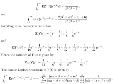
Note that ifm= 2λthenX1has the same mean as the exponential random variable with parameterλ(exp(λ)). Form= 1, using Theorem 4.2. we obtain

Z ∞ Inverting these transforms we obtain

E[Y(t)] = 1

Hence the variance ofY(t) is given by

Var[Y(t)] = 1

The double Laplace transform ofY(t) is given by

Z ∞

The pdf of Y(t) can be approximated by first truncating the infinite sum in this transform and then by inverting the truncated transform. The graph of the pdf of Y(3) form= 1 can be seen in Figure 1 (dashed line).

(11)

REFERENCES

1. J. Abate and W. Whitt_{, ”The Fourier-series method for inverting transforms of} probability distributions”,Queuing Systems10(1992), 5–88.

2. I.S. Gradshteyn and I.M. Ryzhik_,Table of Integrals, Series, and Products, Academic Press, London, 1994.

3. J. Grandell,Doubly Stochastic Poisson Processes, Springer-Verlag, Berlin, 1943. 4. J.A. Gubner_{, ”Computation of shot-noise probability distributions and densities”,}

SIAM Journal on Scientific Computing17 (3)(1993), 750–761.

5. S.I. Resnick, Extreme Values, Regular Variation, and Point Processes, Springer-Verlag, Berlin, 1987.

6. S.M. Ross_,Stochastic Processes, John Wiley, New York, 1996.

7. Suyono and J.A.M. van der Weide_{, ”Asymptotic properties of integrated renewal} processes”,Presented at the SEAMS-GMU Conference, (2007).

8. D.V. Widder,The Laplace transform, Princeton University Press, Princeton, 1946.

Suyono_{: Jurusan Matematika FMIPA Universitas Negeri Jakarta 13200, Indonesia.} E-mail: [email protected]

J.A.M. van der Weide_{: Delft University of Technology, Hb. 06.150, Mekelweg 4, 2624}

CD Delft, The Netherlands.