STRUCTURED CONDITION NUMBERS
AND BACKWARD ERRORS IN SCALAR PRODUCT SPACES∗
FRANC¸ OISE TISSEUR† AND STEF GRAILLAT‡
Abstract. The effect of structure-preserving perturbations on the solution to a linear sys-tem, matrix inversion, and distance to singularity is investigated. Particular attention is paid to linear and nonlinear structures that form Lie algebras, Jordan algebras and automorphism groups of ascalar product. These include complex symmetric, pseudo-symmetric, persymmetric, skew-symmetric, Hamiltonian, unitary, complex orthogonal and symplectic matrices. Under reasonable assumptions on the scalar product, it is shown that there is little or no difference between structured and unstructured condition numbers and distance to singularity for matrices in Lie and Jordan alge-bras. Hence, for these classes of matrices, the usual unstructured perturbation analysis is sufficient. It is shown that this is not true in general for structures in automorphism groups. Bounds and com-putable expressions for the structured condition numbers for a linear system and matrix inversion are derived for these nonlinear structures.
Structured backward errors for the approximate solution of linear systems are also considered. Conditions are given for the structured backward error to be finite. For Lie and Jordan algebras it is proved that, whenever the structured backward error is finite, it is within a small factor of or equal to the unstructured one. The same conclusion holds for orthogonal and unitary structures but cannot easily be extended to other matrix groups.
This work extends and unifies earlier analyses.
Key words. Structured matrices, Normwise structured perturbations, Structured linear sys-tems, Condition number, Backward error, Distance to singularity, Lie algebra, Jordan algebra, Au-tomorphism group, Scalar product, Bilinear form, Sesquilinear form, Orthosymmetric.
AMS subject classifications. 15A12, 65F35, 65F15.
1. Motivations. Condition numbers and backward errors play an important role in numerical linear algebra. Condition numbers measure the sensitivity of the solution of a problem to perturbation in the data whereas backward errors reveal the stability of a numerical method. Also, when combined with a backward error estimate, condition numbers provide an approximate upper bound on the error in a computed solution.
There is a growing interest in structured perturbation analysis (see for example [1], [6], [15] and the literature cited therein) due to the substantial development of algorithms for structured problems. For these problems it is often more appropriate to define condition numbers that measure the sensitivity to structured perturbations. Structured perturbations are not always as easy to handle as unstructured ones and the backward error analysis of an algorithm is generally more difficult when structured perturbations are concerned. Our aim in this paper is to identify classes of
∗Received by the editors 19 September 2005. Accepted for publication 16 April 2006. Handling
Editor: AngelikaBunse-Gerstner.
†School of Mathematics, The University of Manchester, Sackville Street, Manchester, M60 1QD,
UK ([email protected],http://www.ma.man.ac.uk/~ftisseur/). This work was supported by Engineering and Physical Sciences Research Council grant GR/S31693.
‡Laboratoire LP2A, Universit´e de Perpignan Via Domitia, 52, avenue Paul Alduy, F-66860
Per-pignan Cedex, France ([email protected],http://gala.univ-perp.fr/~graillat/).
matrices for which the ratio between the structured and the unstructured condition number of a problem and the ratio between the structured and unstructured back-ward error are close to one. For example, it is well-known that for symmetric linear systems and for normwise distances it makes no difference to the backward error or condition number whether matrix perturbations are restricted to be symmetric or not [1], [5], [16]. Rump [15] recently showed that the same holds for skew-symmetric and persymmetric structures. We unify and extend these results to a large class of structured matrices.
The structured matrices we consider belong to Lie and Jordan algebras or group automorphisms associated with unitary and orthosymmetric scalar products. These include for example symmetric, complex symmetric and complex skew-symmetric matrices, pseudo-symmetric, persymmetric and perskew-symmetric matrices, Hamil-tonian and skew-HamilHamil-tonian matrices, Hermitian, skew-Hermitian andJ-Hermitian matrices, but also nonlinear structures such as orthogonal, complex orthogonal, sym-plectic, unitary and conjugate symplectic structures. Structures not in the scope of our work include Toeplitz, Hankel and circulant structures, which are treated by Rump [15].
The paper is organized as follows. In Section 2, we set up the notation and re-call some necessary background material. In Section 3, we consider the condition number for the matrix inverse and the condition number for linear systems as well as the distance to singularity. We show that for matrices belonging to Lie or Jordan algebras associated with a unitary and orthosymmetric scalar product and for pertur-bations measured in the Frobenius norm or 2-norm, the structured and unstructured condition numbers are equal or within a small factor of each other and that the dis-tance to singularity is unchanged when the perturbations are forced to be structured. Hence, for these classes of matrices the usual unstructured perturbation analysis is sufficient. We show that this is false in general for nonlinear structures belonging to automorphism groups. We give bounds and derive computable expressions for the matrix inversion and linear system structured condition numbers. Structured back-ward errors for linear systems are considered in Section 4. Unlike in the unstructured case, the structured backward error may not exist and we say in this case that it is infinite. We give conditions on b and the approximate solutionxto Ax=b for the structured backward error to be finite. We show that for Lie and Jordan algebras of orthosymmetric and unitary scalar products when the structured backward error is finite it is within a small factor of the unstructured one. Unfortunately, there is no general technique to derive explicit expressions for the structured backward error for structures in automorphism groups. For orthogonal and unitary matrices, we show that the Frobenius norm structured backward error when it exists differs from the unstructured one by at most a factor√2.
2. Preliminaries. We begin with the basic definitions and properties of scalar products and the structured classes of matrices associated with them. Then we give auxiliary results for these structured matrices.
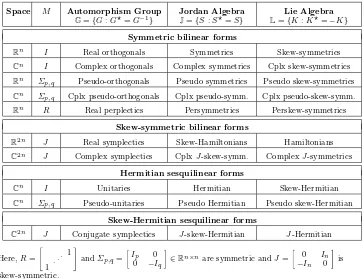
Table 2.1
A sampling of structured matrices associated with scalar products·,·M, whereMis the matrix defining the scalar product.
Space M Automorphism Group Jordan Algebra Lie Algebra
G={G:G⋆=G−1} J={S:S⋆=S} L={K:K⋆=−K}
Symmetric bilinear forms
Rn I Real orthogonals Symmetrics Skew-symmetrics
Cn I Complex orthogonals Complex symmetrics Cplx skew-symmetrics
Rn Σ
p,q Pseudo-orthogonals Pseudo symmetrics Pseudo skew-symmetrics
Cn Σ
p,q Cplx pseudo-orthogonals Cplx pseudo-symm. Cplx pseudo-skew-symm.
Rn R Real perplectics Persymmetrics Perskew-symmetrics
Skew-symmetric bilinear forms
R2n J Real symplectics Skew-Hamiltonians Hamiltonians
C2n J Complex symplectics CplxJ-skew-symm. ComplexJ-symmetrics
Hermitian sesquilinear forms
Cn I Unitaries Hermitian Skew-Hermitian
Cn Σ
p,q Pseudo-unitaries Pseudo Hermitian Pseudo skew-Hermitian
Skew-Hermitian sesquilinear forms
C2n J Conjugate symplectics J-skew-Hermitian J-Hermitian
Here,R=
" 1 . .. 1
#
andΣp,q=
Ip 0 0 −Iq
∈Rn×nare symmetric andJ=
0 In
−In 0
is
skew-symmetric.
Kn. Here K denotes the field R or C. It is well known that any real or complex
bilinear form·,·has a unique matrix representation given by ·,·=xTM y, while
a sesquilinear form can be represented by ·,· = x∗M y, where the matrix M is nonsingular. We will denote·,·by·,·M as needed.
A bilinear form is symmetric if x, y = y, x, and skew-symmetric if x, y = −y, x. Hence for a symmetric form M = MT and for a skew-symmetric form
M =−MT. A sesquilinear form is Hermitian ifx, y=y, xand skew-Hermitian if
x, y=−y, x. The matrices associated with such forms are Hermitian and skew-Hermitian, respectively.
To each scalar product there corresponds a notion ofadjoint, generalizing the idea of transposeT and conjugate transpose∗, that is, for any matrixA∈Kn×n there is
a unique adjointA⋆with respect to the form defined byAx, yM=x, A⋆yM for all
xandy in Kn. In matrix terms the adjoint is given by
A⋆=
M−1ATM for bilinear forms,
M−1A∗M for sesquilinear forms. (2.1)
Jand the automorphism group Gdefined by
L=L∈Kn×n:Lx, yM =−x, LyM
=L∈Kn×n:L⋆=−L, J= S∈Kn×n:Sx, yM =x, SyM
=S∈Kn×n:S⋆=S, G= G∈Kn×n:Gx, Gy
M=x, yM
={G∈Kn×n : G⋆=G−1}. The setsLandJ are linear subspaces. They are not closed under multiplication but are closed under inversion: if A ∈ S is nonsingular, where S = L or S = J then A−1∈S. Matrices inGform a Lie group under multiplication.
There are two important classes of scalar products termed unitary and orthosym-metric [13]. The scalar product·,·M isunitary ifαM is unitary for some α >0. A
scalar product is orthosymmetric if
M =
βMT, β=±1, (bilinear forms),
βM∗, |β|= 1, (sesquilinear forms).
(See [13, Definitions A.4 and A.6]for a list of equivalent properties.) One can show that up to a scalar multiple there are only three distinct types of orthosymmetric scalar products: symmetric and skew-symmetric bilinear, and Hermitian sesquilinear [14]. We will, however, continue to include separately stated results (without separate proofs) for skew-Hermitian forms for convenience, as this is a commonly occurring special case.
In the rest of this paper we concentrate on structured matrices in the Lie algebra, the Jordan algebra or the automorphism group of a scalar product which is both unitary and orthosymmetric. These include, but are not restricted to, the structured matrices listed in Table 2.1, all of which correspond to a unitary and orthosymmetric scalar product with α= 1 and β=±1.
2.2. Auxiliary results. The characterization of various structured condition numbers and backward errors for linear systems relies on the solution to the following problem: Given a class of structured matricesS, for which vectorsx, bdoes there exist someA∈Ssuch thatAx=b? Mackey, Mackey and Tisseur [14], [12] give a solution for this problem whenSis the Lie algebra, Jordan algebra or automorphism group of an orthosymmetric scalar product. Here and below we writeı=√−1.
Theorem 2.1 ([14, Thm. 3.2]and [12]). Let S be the Lie algebra L, Jordan algebra J or automorphism group G of an orthosymmetric scalar product ·,·M on
Kn. Then for any given pair of vectorsx,b∈Kn withx= 0, there existsA∈Ssuch that Ax=b if and only if the conditions given in the following table hold:
Bilinear forms Sesquilinear forms
S
Symmetric Skew-symmetric Hermitian Skew-Hermitian
In what follows · ν denotes as the 2-norm · 2 or the Frobenius norm · F.
The next result will be useful.
Theorem 2.2. LetSbe the Lie or Jordan algebra of a scalar product·,·M which
is both orthosymmetric and unitary and letx, b∈Kn of unit2-norm be such that the relevant condition in Theorem 2.1is satisfied. Then,
min{Aν:A∈S, Ax=b}=
1 if ν= 2,
2−α2b, x2
M if ν=F,
whereαis such that αM is unitary. Proof. See [14, Thms 5.6 and 5.10].
Note that when it exists, the minimal Frobenius norm solutionAopt to Ax=b
withA∈S is unique and is given by
Aopt=
bx∗ x∗x+ǫ
bx∗ x∗x
⋆ I−xx
∗ x∗x
, ǫ=
1 ifS=J, −1 ifS=L,
where⋆is the adjoint with respect to the scalar product ·,·M associated withS.
The next lemma shows that whenSis the Lie or Jordan algebra of an orthosym-metric scalar product ·,·M on K
n, left multiplication by M maps S to the sets
Skew(K) and Sym(K) for bilinear forms and, to a scalar multiple of Herm(C) for sesquilinear forms, where
Sym(K) ={A∈Kn×n:AT =A}, Skew(K) ={A∈Kn×n:AT =−A},
(2.2)
Herm(C) ={A∈Cn×n:A∗=A}
are the sets of symmetric and skew-symmetric matrices onKn×nand Hermitian matri-ces, respectively. This is a key result for our unified treatment of structured condition numbers and backward errors.
Lemma 2.3 ([14, Lem. 5.9]). Let Sbe the Lie or Jordan algebra of an orthosym-metric scalar product·,·M. SupposeA∈S, so thatA⋆=δA whereδ=±1.
• For bilinear forms on Kn (K=R,C)write, by orthosymmetry, M =βMT withβ =±1. Then
M·S=
Sym(K) if δ=β, Skew(K) if δ=β. (2.3)
• For sesquilinear forms onCn write, by orthosymmetry,M =βM∗with|β|= 1. Then
M·S=
β1/2Herm(C) if δ= +1,
β1/2ıHerm(C) if δ=−1.
(2.4)
with A. For instance, if A is pseudosymmetric then M = Σp,q = I0p−0Iq
and
A=Σp,qAis symmetric. Then we can use a block LDLT factorization [8, Ch.11]to
solve the modified linear systemAx =Σp,qb. However, since left multiplication ofA
byM changes its spectrum, mapping A to Amay not be appropriate when solving large sparse systems of equations with an iterative method.
2.3. Nearest structured matrix. SupposeAhas lost its structure, because of errors in its construction for example. An interesting optimization problem is to find the nearest structured matrix toA,
dS(A) := min{A−S: S∈S}.
(2.5)
This problem is easy to solve when Sis the Jordan algebra J or Lie algebraL of an orthosymmetric and unitary scalar product·,·M and · is any unitarily invariant
norm. Indeed, if ·,·M is orthosymmetric then any A ∈K
n×n can be expressed in
the form
A= A+A⋆
2 +
A−A⋆
2 =:AJ+AL, whereAJ ∈JandAL∈L. For anyS∈J, so that,S=S⋆we have
A−AJ=AL=
1
2A−A⋆= 1
2(A−S) + (S⋆−A⋆). Since·,·M is unitary and the norm is unitarily invariant,
A−AJ ≤
1
2A−S+ 1
2(S−A)
⋆=A−S ∀S∈J.
We find similarly that for Lie algebrasL,
A−AL ≤ A−S ∀S∈L.
Hence,S=ASwithS=JorLis the nearest structured matrix inSto Aand
dJ(A) =
1
2A−A⋆, dL(A) = 1
2A+A⋆.
Fan and Hoffman solved this problem for the class of symmetric matrices [3]. More recently it was solved by Cardoso, Kenney and Leite [2, Thm. 5.3]for Lie and Jordan algebras of bilinear scalar products·,·M for whichM M
T =I andM2=±I; these
scalar products are a subset of the unitary and orthosymmetric scalar products. WhenSis the set of real orthogonal matrices or unitary matrices, the solution to the nearness problem (2.5) is well-known for the Frobenius norm and is given by
dS(A) =A−UF,
3. Structured condition numbers. We consider normwise relative structured condition numbers that measure the sensitivity of linear systems and of matrix inver-sion, and investigate the structured distance to singularity.
3.1. Linear systems. LetS be a class of structured matrices, not necessarily J,LorG. We define the structured normwise condition number for the linear system Ax=b withx= 0 by
cond(A, x;S) = lim
ǫ→0sup
∆x
ǫx : (A+∆A)(x+∆x) =b+∆b, (3.1)
A+∆A∈S, ∆A ≤ǫA, ∆b ≤ǫb
,
where · is an arbitrary matrix norm. Let cond(A, x)≡cond(A, x;Kn×n) denote
the unstructured condition number, wherenis the dimension ofA. Clearly,
cond(A, x;S)≤cond(A, x).
If this inequality is not always close to being attained then cond(A, x) may severely overestimate the worst case effect of structured perturbations.
Let us define for nonsingularA∈Sand nonzerox∈Kn,
φ(A, x;S) = lim
ǫ→0sup
A−1∆Ax
ǫA : ∆A ≤ǫA, A+∆A∈S
. (3.2)
We write φ(A, x) ≡ φ(A, x;Kn×n) when A+∆A is unstructured and φ
2(A, x) or
φF(A, x) to specify that the 2-norm or Frobenius norm is used in (3.2). Similarly,
cond2and condF mean that · = · 2or · = · F in (3.1).
The next lemma is useful when comparing the structured and unstructured con-dition numbers for linear systems. The result is due to Rump [15]and holds for any class of structured matrices. The proof in [15, Thm. 3.2 and Thm. 33]forK=Rand the 2-norm extend trivially toK=Cand · = · F.
Lemma 3.1. Let A ∈ Kn×n be nonsingular and x∈ Kn be nonzero. Then for
ν= 2, F,
φν(A, x;S)
x2
Aν+
b2
x2
≤condν(A, x;S)≤ A−12
Aν+
b2
x2
.
and
condν(A, x,S) =c
φν(A, x;S)Aν
x2
+A −1
2b2
x2
, √1
2 ≤c≤1.
in (3.2) is attained by ∆A = ǫAνyx∗/x2, where y is such that y2 = 1 and
A−1y
2=A−12. This implies the well known formula
φ2(A, x) =φF(A, x) =A−12x2,
(3.3)
so that from the first part of Lemma 3.1,
condν(A, x) =A−12Aν+
A−1
2b2
x2
, ν= 2, F. (3.4)
The rest of this section is devoted to the study of φ(A, x;S) for the structured matrices inL,J orGas defined in Section 2.1.
3.1.1. Lie and Jordan algebras. D. J. Higham [5]proves that for real sym-metric structures,
condν(A, x; Sym(R)) = condν(A, x), ν = 2, F
and Rump [15]shows that equality also holds in the 2-norm for persymmetric and skew-symmetric structures. These are examples of Lie and Jordan algebras (see Table 2.1). We extend these results to all Lie and Jordan algebras of orthosymmetric and unitary scalar products. Unlike the proofs in [15], our unifying proof does not need to consider each algebra individually.
Theorem 3.2. Let S be the Lie algebra or Jordan algebra of a unitary and orthosymmetric scalar product ·,·M on K
n. For nonsingular A ∈ S and nonzero
x∈Kn, we have
φ2(A, x;S) =φ2(A, x),
1 √
2φF(A, x)≤φF(A, x;S)≤φF(A, x).
Proof. Clearlyφν(A, x;S) ≤φν(A, x). Since Lie and Jordan algebras are linear
subspaces ofKn×n,φν(A, x,S) can be rewritten as
φν(A, x;S) = supA−1∆Ax2: ∆Aν ≤1, ∆A∈S.
Suppose that there exists u∈Kn of unit 2-norm such that A−1u
2 =A−12 and
such that the pair (x/x2, u) satisfies the relevant condition in Theorem 2.1. Then
Theorem 2.2 tells us that there exist E2, EF ∈ S such that Eνx=x2u, ν = 2, F
andE22= 1,EFF ≤
√
2. Thus
φν(A, x) =A−12x2=A−1u2x2=A−1Eνx2≤cνφν(A, x;S),
withc2= 1 and cF =
√
2 and the statement of the Theorem follows.
To complete the proof we need to show that there is always a vector u such that A−1u
2 = A−12 and such that x/x2, u satisfy the relevant condition in
(i) For bilinear forms, orthosymmetry of the scalar product implies thatMT =
βM,β=±1. Ifδ=β, Theorem 2.1 says that there is no condition onxandufor the existence of a structured matrix mappingxtox2u, soucan be any singular vector
ofA−1 associated with the largest singular value. Ifδ=β thenxandumust satisfy
u, xM = 0. But [13, Thm. 8.4]says that the singular values ofAand thereforeA
−1
all have even multiplicity. Hence there exits orthogonal vectorsu1andu2in Kn such
thatu12=u22= 1 andA−1u12=A−1u22=A−12. Letu∈span{u1, u2}
such thatu, xM =u
TM x= 0 and u
2= 1. Then necessarily,A−1u2=A−12.
(ii) For sesquilinear forms, since singular vectorsu are defined up to a nonzero scalar multiple, we choose u to be the singular vector associated with the largest singular value ofA−1 and such that the condition in Theorem 2.1 is satisfied.
Lemma 3.1 and Theorem 3.2 together yield the following result.
Theorem 3.3. Let S be the Lie or Jordan algebra of a unitary and orthosym-metric scalar product·,·M onK
n. LetA
∈Sbe nonsingular and x∈Kn with x= 0
be given. Then
cond2(A, x;S) = cond2(A, x),
1 √
2condF(A, x)≤condF(A, x;S)≤condF(A, x).
We conclude from Theorem 3.3 that for many Lie and Jordan algebras, the con-straintA+∆A∈S has little or no effect on the condition number. This is certainly true for all the examples in Table 2.1.
3.1.2. Automorphism groups. WhenSis a smooth manifold the task of com-puting the supremum (3.2) simplifies to a linearly constrained optimization problem. This was already observed by Karow, Kressner and Tisseur in [10]for a different supremum.
Lemma 3.4. Let S be a smooth real or complex manifold. Then for A ∈ S
nonsingular we have
φ(A, x;S) = supA−1Ex: E= 1, E∈TAS,
(3.5)
whereTAS is the tangent space atA.
Proof. Let E∈TASwith E= 1. Then there is a smooth curvegE : (−ǫ, ǫ)→
Kn×n satisfyingg
E(0) = 0,g′E(0) =E andA+gE(t)∈Sfor allt. We have
lim
t→0
gE(t)
gE(t)
= lim
t→0
Et+O(|t|2)
Et+O(|t|2) =E.
Hence
lim
t→0
A−1g
E(t)x
gE(t)
=A−1Ex.
This impliesφ(A, x;S)≥supA−1Ex: E= 1, E∈T
AS.Equality holds since
the union of the curvesA+gE contains an open neighborhood inSofA(see [10]for
An automorphism groupGforms a smooth manifold. DefineF(A) =A⋆A−Iso that A∈Gis equivalent to F(A) = 0. The tangent space TAGatA∈Gis given by
the kernel of the Fr´echet derivativeJA ofF atA:
TAG={X ∈Kn×n:JA(X) = 0}
={X ∈Kn×n:A⋆X+XA= 0} ={AH∈Kn×n:H⋆=−H} =A·L,
(3.6)
whereLis the Lie algebra of·,·M.
ForS=G, the supremum (3.5) can then be rewritten as
φ(A, x;G) = sup{Hx: AH= 1, H ∈L}. (3.7)
In a similar way to [6]and [10], an explicit expression for φ(A, x;G) can be obtained for the Frobenius norm. Let us rewrite
Hx= (xT⊗In)vec(H),
where ⊗ denotes the Kronecker product and vec is the operator that stacks the columns of a matrix into one long vector. We refer to Lancaster and Tismenetsky [11, Chap. 12]for properties of the vec operator and the Kronecker product. SinceL is a linear vector space of dimensionm≤n2, there is ann2×mmatrixB such that
for everyH ∈Lthere exists a uniquely defined parameter vectorqwith
vec(H) =Bq. (3.8)
Let (I⊗A)B=QRbe a reduced QR factorization of (I⊗A)B, i.e.,Q∈Kn2×m, R∈ Km×m, and letp=Rq. Then,
vec(AH) = (I⊗A)vec(H) = (I⊗A)Bq=Qp
so thatAHF =vec(AH)2=p2and
Hx= (xT⊗In)vec(H) = (xT⊗In)(I⊗A)−1vec(AH) = (xT⊗A−1)Qp.
Hence (3.7) becomes
φF(A, x;G) = sup(xT⊗A−1)Qp2: p2= 1, p∈Km=(xT⊗A−1)Q2.
Using the last part of Lemma 3.1 we then have, up to a small scalar multiple, a directly computable expression for the structured condition number.
Theorem 3.5. Let Gbe the automorphism group of any scalar product and let
Lbe the associated Lie algebra. Then
condF(A, x,G) =c
(xT⊗A−1)Q2
AF
x2 +
A−1
2b2
x2
, √1
where(I⊗A)B=QRis a reduced QR factorization of(I⊗A)B andB is a pattern matrix for Lin the sense of(3.8).
The expression for condF(A, x;G) in Theorem 3.5 has two disadvantages. First,
it is expensive to compute, since it requires the QR factorization of ann2×mmatrix.
Note that sinceA∈G,A−1=A⋆withA⋆given in (2.1) so that we do not necessarily
need to invertA. Second, it is difficult to compare with the unstructured condition number condF(A, x) in (3.4). However, when ·,·M is unitary and orthosymmetric,
we can bound the ratioφν(A, x;G)/φν(A, x) from below.
Lemma 3.6. LetGbe the automorphism group of a unitary and orthosymmetric scalar product onKn. LetA∈Gandx∈Kn with x= 0 be given. Then
cν φν(A, x)
A2A−12 ≤φν(A, x;
G)≤φν(A, x), cν=
1 if ν= 2,
1 √
2 if ν=F.
Proof. We just need to prove the lower bound. Let u∈Kn be of unit 2-norm and
such thatxand usatisfy the relevant condition in Theorem 2.1. From Theorem 2.2, there existsS2 ∈Sand SF ∈S such that Sν(x/x2) =u, ν = 2, F andS22 = 1,
SFF ≤
√
2. Let Hν =ξSν ∈S withξ >0 such that AHνν = 1,ν = 2, F. This
impliesξ≥ 1
A2Sνν. Hence from (3.7), we have
φν(A, x;G)≥ Hνx2=ξx2≥
φν(A, x)
A2A−12Sνν
.
Lemma 3.6, together with Lemma 3.1 and the explicit expression for condν(A, x)
in (3.4), yield bounds for cond(A, x;G).
Theorem 3.7. Let Gbe the automorphism group of a unitary and orthosymmet-ric scalar product onKn. LetA∈Gandx∈Kn withx= 0be given. Then
cν
condν(A, x)
A2A−12 ≤
condν(A, x;G)≤condν(A, x), cν=
1 if ν= 2,
1 √
2 if ν=F.
Theorem 3.7 shows that when A is well-conditioned (i.e., A2A−12 ≈ 1),
the structured and unstructured condition numbers for Ax=b are equal or nearly equal. This is the case for the real orthogonal group and the unitary group. For ill-conditionedA, the bounds may not be sharp, as illustrated by the following example. Suppose thatM =J and that·,·J is a real bilinear form. ThenGis the set of real
symplectic matrices (see Table 2.1). Consider the symplectic matrix
A=
D D 0 D−1
, D= diag(10−6,102,2) (3.9)
and define the ratio
ρ= condF(A, x;G)/condF(A, x)
computable expression in Theorem 3.5 with cF = 1 to approximate condF(A, x;G).
Forx= [1,0,0.1,0,0.1,−1]T we obtainρ≈8×10⁻⁵ showing that cond
F(A, x;G)≪
condF(A, x) may happen.
3.2. Matrix inversion. LetSbe a class of structured matrices. The structured condition number for the matrix inverse can be defined by
κ(A;S) = lim
ǫ→0sup
(A+∆A)−1−A−1
ǫA−1 : A+∆A∈S, ∆A ≤ǫA
. (3.10)
When∆Ais unstructured we writeκ(A)≡κ(A;Kn×n). It is well-known that for the 2- and Frobenius normsκ(A) has the characterization
κ2(A) =A2A−12, κF(A) =
AFA−122
A−1
F .
(3.11)
See [8, Thm. 6.4]forκ2 and [5]forκF. Again, whenS is a smooth manifold (3.10)
simplifies to a linearly constrained optimization problem.
Lemma 3.8. Let S be a smooth real or complex manifold. Then for A ∈ S
nonsingular we have
κ(A;S) = A
A−1sup{A
−1EA−1: E= 1, E∈T
AS},
(3.12)
whereTASis the tangent space at A.
Proof. The proof is similar to that of Lemma 3.4 and makes use of the expansion
(A+∆A)−1−A−1=−A−1∆AA−1+O(∆A2), in the definition ofκ(A;S) in (3.10).
When S is the Lie algebra or Jordan algebra of a scalar product, the tangent space atSisSitself: TAS=S. If we restrict·,·M to be orthosymmetric and unitary
then there is equality between the structured and unstructured condition numbers for both the 2-norm and Frobenius norm.
Theorem 3.9. Let S be the Lie algebra or Jordan algebra of a unitary and orthosymmetric scalar product ·,·M onK
n. For nonsingularA∈S we have
κν(A;S) =κν(A), ν = 2, F.
Proof. Using the inequalityABCν≤ A2BνC2 in (3.12) gives
κν(A;S)≤ AνA−122/A−1ν =κν(A).
SinceαM is unitary for someα >0, we haveκν(A;S) =κν(A; M·S) withA=αM A.
Now assume that there existsE∈M·Ssuch that
Eν = 1, A−1EA−1ν=A−122.
Then (3.12) implies
κ(A, M ·S)≥ Aν A−1
ν
A−1EA−1ν= Aν
A−1
νA
−1
22=κν(A).
Hence to complete the proof we just need to construct E ∈ M·S satisfying (3.13). Since the scalar product is orthosymmetric, we have from Lemma 2.3 that M·S is one of Sym(K), Skew(K) and Herm(C).
(i) M·S = Sym(K). Let A−1 = U ΣUT be the Takagi factorization of A−1 ∈
Sym(K), whereU is unitary andΣ= diag(σ1, σ2, . . . , σn) withA−12=σ1≥σ2≥
· · · ≥σn≥0 [9, Cor. 4.4.4]. When K=R, U is orthogonal andA−1=U ΣUT is the
singular value decomposition ofA−1. TakeE= ¯U e1eT1U∗.
(ii) M·S = Skew(K). We consider the skew-symmetric analog of the Takagi factorization (Problems 25 and 26 in [9, Sec. 4.4]). Since A−1 ∈ Skew(K), there
exists a unitary matrix U such that A−1 = U DUT where D = D
1⊕ · · · ⊕Dn/2,
with Dj = −0zj +zj
0
, 0 = zj ∈ C, j = 1:n/2. When K = R, U is orthogonal.
Assume that the zj are ordered such that A−12 =|z1| ≥ |z2| ≥ · · · ≥ |zk|. Take
E=cνU(e¯ 1eT2 −e2eT1)U∗,ν = 2, F withc2= 1 and cF = 1/
√ 2.
(iii)M·S= Herm(C). TakeE =U e1e∗1U∗ where U is the unitary factor in the
singular value decomposition ofA−1.
When S is the automorphism group G of a scalar product there is a directly computable expression forκF(A;G). Its derivation is similar to that of cond(A, x;G)
described in section 3.1.2.
Theorem 3.10. Let Gbe the automorphism group of any scalar product and let
Lbe the associated Lie algebra. Then
κF(A;G) =
AF
A−1
F
(AT ⊗A)−1Q2.
where(I⊗A)B=QRis a reduced QR factorization of(I⊗A)B andB is a pattern matrix for Lin the sense of(3.8).
It is well-known that κ2(A) ≥ 1. This is also true for κ2(A;G) when G is the
automorphism group of a unitary and orthosymmetric scalar product. Indeed let u, v∈Kn be such thatA−1u=A−1
2v withu2=v2 = 1. Then, from (3.12),
(3.6) and (3.7),
κ2(A;G) =
A2
A−1 2
sup{HA−1
2:AH2= 1, H∈L}
≥ A2 A−1
2A
−1
2sup{Hv2:AH2= 1, H∈L}
=A2φ2(A, v;G).
But from Lemma 3.6,φ2(A, v;G)≥1/A2so that
Clearly, if A is well conditioned then κ2(A;G) ≈ κ2(A). This is certainly true for
the orthogonal and unitary groups. For the symplectic matrixAdefined in (3.9), we find that κF(A;G) ≈ κ2(A;G) = 1.0001 but that κ2(A) = 1×10
12, showing that
κ2(A;G)≪κ2(A) may happen.
3.3. Nearness to singularity. Thestructured distance to singularity of a ma-trix is defined by
δ(A;S) = minǫ: ∆A ≤ǫA, A+∆Asingular, A+∆A∈S. (3.14)
D. J. Higham [5]showed that for symmetric perturbations,
δν(A; Sym(R)) =δν(A), ν= 2, F,
so that the constraint∆A=∆AT has no effect on the distance. This is a special case
of the following more general result.
Theorem 3.11. Let S be the Lie or Jordan algebra of a unitary and orthosym-metric scalar product. Let nonsingularA∈S be given. Then
δ2(A;S) =δ2(A),
1 √
2δF(A)≤δF(A;S)≤δF(A).
Proof. It is well-known that the relative distance to singularity is the reciprocal of the condition numberκ(A) or a scalar multiple of it [8, p.111]. Clearly,δν(A;S)≥
δν(A).
Since the scalar product ·,·M is unitary, αM is unitary for some α > 0 and
we have δν(A;S) = δν(A, S), where A = αM A and S = M·S. Since the scalar
product is orthosymmetric we have from Lemma 2.3 thatSis one of Sym(K), Skew(K) and βHerm(C) with |β| = 1. Without loss of generality, assume that Aν = 1.
Since (A+∆A)−1 = (I+A−1∆A) −1A−1 we just need to find ∆A ∈ M·S such
that I+A−1∆A is singular and ∆A
ν ≤ 1/A−12. This is achieved by taking
∆A=−E/A−1
2, whereE is the perturbation used in the proof of Theorem 3.9.
Matrices in automorphism groups are nonsingular soδ(A;G) =∞. This ends our treatment of various structured condition numbers.
4. Normwise structured backward errors. When solving a linear system Ax = b with A ∈ S ⊂ Kn×n, one is interested in whether a computed solution x
solves a nearby structured system: for example whether the particular structured backward error
µ(x;S) = min{∆A: (A+∆A)x=b, A+∆A∈S} (4.1)
is relatively small. Note that in (4.1), only the coefficient matrixAis perturbed. Let ∆Aopt be an optimal solution defined by ∆Aopt =µ(x; S) and let r=b−Axbe
the residual vector. It is well known that for unstructured perturbations,
and this is achieved by∆Aopt =rx∗/(x∗x). Unlike the unstructured case, there may
not be any solution∆Ato (A+∆A)x=b withA+∆A∈S. In this case we write that µ(x; S) = ∞. If one uses a structure preserving algorithm to solve the linear system thenA+∆Ais structured and the backward error is guaranteed to be finite. This may not be the case if the system is solved using a linear solver that does not take advantage of the structure even if it is backward stable.
When bothAandb are perturbed we define the corresponding structured back-ward error by
η(x; S) = min{ǫ: (A+∆A)x=b+∆b, A+∆A∈S, (4.2)
∆A ≤ǫA, ∆b ≤ǫb}.
Again, for unstructured perturbations we have the well-known explicit expression [8, Thm. 7.1],
ην(x)≡η(x;Kn×n) =
r2
Aνx2+b2
, ν= 2, F. (4.3)
The structured backward error η(x;S) is harder to analyze than µ(x;S). The con-straint A+∆A ∈ S generally implies an extra constraint on the perturbation ∆b. For example, if S = Skew(R) then for there to exist ∆Askew-symmetric such that (A+∆A)x=b+∆bone needsxT(b+∆b) = 0 (see Theorem 2.1). On the other hand
one may have η(x;S) finite but µ(x; S) = ∞. The next theorem shows that when the particular backward errorµ(x;S) exists, its study provides useful information on η(x;S).
Theorem 4.1. LetA∈S, whereSis a class of structured matrices and letx= 0
be an approximate solution to Ax =b. If µν(x; S) is finite with µν(x; S)≤cνµν(x) then for ην(x)<1,
ην(x) ≤ην(x; S)≤
2cν ην(x)
1−ην(x)
, ν = 2, F. (4.4)
Proof. The proof is modelled from the solution to [8, Exercise 7.7]concerning the unstructured case. Clearly, from the definitions ofην(x; S) andµν(x;S),
ην(x) ≤ην(x; S)≤
µν(x; S)
Aν ≤
cν
µν(x)
Aν
=cν
r2
Aνx2
. (4.5)
Letǫ=ην(x). Then from (4.3) we have thatr2≤ǫ(Aνx2+b2) withb2=
(A+∆A)x−∆b2≤(1+ǫ)Aνx2+ǫb2yieldingb2≤(1−ǫ)−1(1+ǫ)Aνx2.
Thus
r2≤
2ǫ
1−ǫAνx2 and (4.5) yields the required bounds.
Theorem 4.1 shows that when ην(x) and cν are small, the structured relative
4.1. Lie and Jordan algebras. For Lie or Jordan algebras (S=Lor J) of a scalar product·,·M the structured backward errorµ(x;S) can be rewritten as
µ(x;S) = min{∆A: ∆Ax=r, ∆A∈S},
wherer=b−Ax. When the scalar product is orthosymmetric and unitary (i.e., αM is unitary for some α >0), Theorem 2.2 implies that forx, b satisfying the relevant condition in Theorem 2.1,
µν(x;S) =
r2
x2 ifν = 2,
2r
2 2
x2 2
−α2|r,xM| 2
x4 2
ifν =F.
Sinceα|r,xM| ≤ r2αMx2=x2r2 the next result follows.
Theorem 4.2. Let S be the Lie algebra or Jordan algebra of an orthosymmetric and unitary scalar product. Let A∈S be nonsingular andx∈Kn be an approximate nonzero solution to Ax=b. If x and b satisfy the conditions in Theorem 2.1 then, for ν= 2, F,
µ2(x; S) =µ2(x),
µF(x)≤µF(x;S)≤
√
2µF(x),
otherwiseµν(x; S) =∞,ν= 2, F.
Theorem 4.2 shows that forcing the backward error matrix to have the structure ofS has either little effect or a drastic effect on its norm. Not all structures require conditions onxand b forµ(x; S) to be finite. For example, for symmetric, complex symmetric, pseudo-symmetric, persymmetric and Hamiltonian structures the struc-tured backward error always exists and is equal to or within a small factor of the unstructured one.
4.2. Automorphism groups. Structured backward errors are difficult to an-alyze for nonlinear structures. Some progress is made in this section for specific automorphism groups. For that we need a characterization of the set of all matrices in the automorphism groupGof an orthosymmetric scalar product mappingxtob.
Theorem 4.3 ([12]). SupposeGis the automorphism group of an orthosymmet-ric scalar product ·,·M, and let x, b, v ∈ K
n such that x, x
M = b, bM =v, vM.
Let Gx, Gb be any fixed elements of G such that Gxx = v and Gbb = v, and let
Gv={Q∈G:Qv=v}. Then
{A∈G:Ax=b}={G⋆bQGx: Q∈Gv}.
(4.6)
The proof in [12]is short and we recall it.
Proof. LetS1={A∈G:Ax=b} andS2={A=G⋆bQGx:Q∈Gv}. Suppose
A∈ S1, and considerQ:=GbAG−x1∈G. ClearlyGbAG−x1v=v, soQ∈Gv. Hence
Conversely, suppose A ∈ S2, so A =Gb−1QGx where Q∈ Gv. Because G is a
group,A∈G. AlsoAx=G−b1QGxx=G−b1Qv=G
−1
b v=b, so A∈ S1.
As a consequence of Theorem 4.3, ifx,xM =b, bM we can rewrite the
struc-tured backward error in (4.1) as
µ(x; G) = min
Q∈GvG⋆bQGxb−A,
(4.7)
where Gbx, Gb are fixed elements of
G satisfying G
b
xx = Gbb = v for some vector
v ∈ Kn, and G
v = {Q ∈ G : Qv = v}. For many of the groups listed in Table
2.1 it is possible to determine explicitly the setGv for some suitably chosen vectors v. For example whenGis the real orthogonal or unitary group, there exist G
b x, Gb
unitary such thatGbxx=x2e1andGbb=b2e1. Sincex2=b2we can choose
v=x2e1giving
Gv={Q∈G:Qe1=e1}=
1 0 0 V
: V∗=V−1∈K(n−1)×(n−1)
.
For these two groups we derive an explicit expression for the structured backward error and show that it is within a small factor of the unstructured one.
In what followsGdenotes either the real orthogonal group or the unitary group. Without loss of generality we assume thatx2=b2= 1. Let Gxbbe any element
of G such that Gxbx = e1 and write G
∗
b x =
x X. Let G ∈ G be the unitary Householder reflector mappingxtob. ThenGb:=GbxG
∗ ∈GsatisfiesG
bb=e1and
G∗
b =
b GX. For anyQ∈Gv withv =e1 the quantity whose norm needs to be
minimized in (4.7) can be rewritten as
G⋆bQGbx−A=G
∗ b 1 V
Gbx−AG
∗
b
xGbx, V
∗=V−1
∈K(n−1)×(n−1) =bx∗+GXV X∗−Ax XGbx
=b−Ax GXV −AXGbx
so that, for the Frobenius norm,µ(x; G) in (4.7) becomes
µF(x;G)2=r22+ min
V∗V=IG
XV −AX2F.
The minimization problem above is a well-known Procrustes problem whose solution is given byGXU −AXF, whereU is the unitary factor of the polar decomposition
ofX∗G∗AX [4, p. 601]. Hence, since Gis unitary, we obtain an explicit expression for the structured backward error,
µF(x; G)2=r22+XU −G∗AX2F.
(4.8)
We now compare the size ofXU −G∗AX
Fto that ofr2using a technique similar
to that of Sun in [17]. Becausex Xis unitary,xx∗+XX∗=I and
XU−G∗AX =X
−x∗G∗AX U −X∗G∗AX
Hence
XU −G∗AX2F =U−X∗G∗AX2F+x∗G∗AX22
=I−H22F+x∗G∗AX22,
(4.9)
where H2 is the Hermitian polar factor of X∗G∗AX. We now need the following
Lemma.
Lemma 4.4 ([17, Lem. 2.4]and [18, Lem. 2.2]). Let A ∈ Cm×m be unitary,
X1 ∈ Cm×k with 2k ≤ m, X = [X1, X2] be unitary, and let H1 and H2 be the
Hermitian polar factors ofX∗
1AX1 andX2∗AX2 respectively. Then, for any unitarily
invariant norm,
I−H1=I−H2 and X1∗AX2=X2∗AX1.
Applying Lemma 4.4 to (4.9) withX1=x, X2=X andG∗Ain place ofAyields
I−H22F+x∗G∗AX22=eıθ−x∗G∗Ax22+X∗G∗Ax22,
(4.10)
whereθ= arg(x∗B∗A
x). Finally, sincex Xis unitary,
x X
eıθ−x∗G∗Ax −X∗G∗A
x
=xeıθ−G∗A
x
so that
eıθ−
x∗G∗A
x2
2+X∗G∗Ax22=xeıθ−G∗Ax22
(4.11)
Hence combining (4.8)–(4.11) givesBU −AXF =xeıθ−G∗Ax2. But
xeıθ−G∗Ax2= min
|ρ|=1xρ −B
∗A
xF ≤ x−B∗AxF =b−Ax2=r2.
We have just proved the following result.
Theorem 4.5. Let Gbe the real orthogonal or unitary matrix group. Let A∈G
andx∈Kn be a nonzero approximate solution toAx=b. Ifx2=b2 then
µF(x) ≤µF(x; G)≤
√
2µF(x),
otherwiseµF(x;G) =∞.
This generalizes Sun’s result on backward errors for the unitary eigenvalue prob-lem, for whichbhas the special form b=eıθx.
REFERENCES
[1] James R. Bunch, James W. Demmel, and Charles F. Van Loan. The strong stability of algo-rithms for solving symmetric linear systems. SIAM J. Matrix Anal. Appl., 10(4):494–499, 1989.
[2] Jo˜ao R. Cardoso, Charles S. Kenney, and F. Silva Leite. Computing the square root and logarithm of a realP-orthogonal matrix. Appl. Numer. Math., 46(2):173–196, 2003. [3] Ky Fan and A. J. Hoffman. Some metric inequalities in the space of matrices. Proc. Amer.
Math. Soc., 6:111–116, 1955.
[4] Gene H. Golub and Charles F. Van Loan. Matrix Computations. Johns Hopkins University Press, Baltimore, MD, USA, third edition, 1996.
[5] Desmond J. Higham. Condition numbers and their condition numbers. Linear Algebra Appl., 214:193–213, 1995.
[6] Desmond J. Higham and Nicholas J. Higham. Backward error and condition of structured linear systems. SIAM J. Matrix Anal. Appl., 13(1):162–175, 1992.
[7] Nicholas J. Higham. Matrix nearness problems and applications. In M. J. C. Gover and S. Barnett, editors, Applications of Matrix Theory, pages 1–27. Oxford University Press, Oxford, 1989.
[8] Nicholas J. Higham. Accuracy and Stability of Numerical Algorithms. Society for Industrial and Applied Mathematics, Philadelphia, PA, USA, second edition, 2002.
[9] Roger A. Horn and Charles R. Johnson. Matrix Analysis. Cambridge University Press, New York, 1985.
[10] Michael Karow, Daniel Kressner, and Fran¸coise Tisseur. Structured eigenvalue condition num-bers. MIMS EPrint 2006.45, Manchester Institute for Mathematical Sciences, The Univer-sity of Manchester, UK, March 2006.
[11] Peter Lancaster and Miron Tismenetsky. The Theory of Matrices. Academic Press, London, second edition, 1985.
[12] D. Steven Mackey, Niloufer Mackey, and Fran¸coise Tisseur. Structured mapping problems for matrices associated with scalar products part II: Automorphism groups. MIMS EPrint, Manchester Institute for Mathematical Sciences, The University of Manchester, UK. In preparation.
[13] D. Steven Mackey, Niloufer Mackey, and Fran¸coise Tisseur. Structured factorizations in scalar product spaces. SIAM J. Matrix Anal. Appl., 27:821–850, 2006.
[14] D. Steven Mackey, Niloufer Mackey, and Fran¸coise Tisseur. Structured mapping problems for matrices associated with scalar products part I: Lie and Jordan algebras. MIMS EPrint 2006.44, Manchester Institute for Mathematical Sciences, The University of Manchester, UK, March 2006.
[15] Siegfried M. Rump. Structured perturbations part I: Normwise distances. SIAM J. Matrix Anal. Appl., 25(1):1–30, 2003.
[16] Ji-guang Sun. On optimal backward perturbation bounds for linear systems and linear least squares problems. Report UMINF 96-15, Department of Computing Science, University of Ume˚a, Sweden, December 1996.
[17] Ji-guang Sun. Backward errors for the unitary eigenproblem. Technical Report UMINF-97.25, Department of Computing Science, University of Ume˚a , Ume˚a, Sweden, 1997.