Ž .
Journal of Health Economics 19 2000 731–753
www.elsevier.nlrlocatereconbase
Consumer satisfaction and supplier
induced demand
Fredrik Carlsen
a,), Jostein Grytten
b aDepartment of Economics, Norwegian UniÕersity of Science and Technology, NTNU,
7491 Trondheim, Norway b
Dental Faculty, UniÕersity of Oslo, Oslo, Norway
Received 4 March 1998; received in revised form 10 February 2000; accepted 2 March 2000
Abstract
This study examines the relationship between supply of primary physicians and con-sumer satisfaction with access to, and quality of, primary physician services in Norway. The purpose is to throw light on a long-standing controversy in the literature on supplier
Ž .
inducement SID : the interpretation of the positive association between physician density and per capita utilization of health services. We find that an increase in the number of physicians leads to improved consumer satisfaction, and that the relationship between satisfaction and physician density exhibits diminishing returns to scale. Our results suggest that policy-makers can compute the socially optimal density of physicians without
knowl-Ž .
edge about whether SID exists, if one accepts the controversial assumption that consumer satisfaction is a valid proxy for patient utility.q2000 Elsevier Science B.V. All rights reserved.
JEL classification: I18
Keywords: Satisfaction; Supplier inducement; Financing; Physicians
1. Introduction
Despite several decades of intensive theoretical and empirical research, the
Ž .
extent of supplier inducement SID and policy implications remain controversial
)Corresponding author. Tel.:q47-73-59-1931; fax:q47-73-59-6954.
Ž .
E-mail address: [email protected] F. Carlsen .
0167-6296r00r$ - see front matterq2000 Elsevier Science B.V. All rights reserved.
Ž .
( )
F. Carlsen, J. GryttenrJournal of Health Economics 19 2000 731–753
732
ŽReinhardt, 1985; Phelps, 1986; Feldman and Sloan, 1988; Rice and Labelle, .
1989 . One reason for the controversy is probably the heavy focus on physicians’
motiÕes, and whether they act as perfect agents for patients. Since most patients do
not have and never will gain medical expertise, we may never be able to discern whether patients would have demanded the amount of care they actually receive if physicians and patients were equally informed.
Ž .
Recently, Labelle et al. 1994 have argued that more attention should be paid to the consequences of SID. If additional health services result in improved health status or better access to health care, then SID may be beneficial to society irrespective of physicians’ motives for generating more services. Along the same
Ž .
lines, Ryan 1992 argues that patient satisfaction may be improved by additional supply of health services, even if the additional services are induced.
Adequate data on the effect of health services on health status are often not available, particularly for primary physician services. Alternative sources of information about the benefits of health care are surveys about consumer satisfac-tion with their health care system. There are at least three reasons why surveys
Ž
may provide valuable information to policy-makers Pascoe, 1983; Ware and .
Davies, 1983; Cleary and McNeil, 1988; Hall and Dornan, 1988 . Firstly, along with improved health status, satisfaction is an ultimate outcome of health care. Secondly, there are several dimensions of health services which patients can observe and evaluate, such as travelling distance, waiting time before an appoint-ment, the physical environment and the interpersonal skills of the staff. Thirdly, satisfaction surveys provide information about patient behaviour. Studies show that satisfied patients are more inclined to comply with recommended treatment and keep appointments and are less inclined to shop around for a doctor than
Ž
dissatisfied patients Kincey et al., 1975; Berkanovic and Marcus, 1976; Linn et .
al., 1982; Marquis et al., 1983; Stewart, 1995 .
This paper employs survey data to study the relationship between supply of primary physician services and consumer satisfaction in Norway. Our study is directly related to the long-standing controversy in the SID literature, about the proper interpretation of the association between physician density and per capita utilization of health services. While most studies find a positive relationship between supply of services and utilization, there is no agreement as to whether this reflects SID by physicians to protect their income, a supply response to unob-served variation in population health or an effect of the price andror volume of
Ž
services on access to and quality of health care Fuchs, 1978; Tussing, 1983; Rossiter and Wilensky, 1984; Stano, 1985; Cromwell and Mitchell, 1986; Feldman
. and Sloan, 1988; Rice and Labelle, 1989; Dranove and Wehner, 1994 .
Being no exception, Norwegian studies of SID have also produced conflicting results. While studies based on aggregate data indicate that SID is present, micro data analyses using patients or physicians as the unit of observation have produced
Ž .
( )
F. Carlsen, J. GryttenrJournal of Health Economics 19 2000 731–753 733
physician services, policy-makers may conclude that SID, if it exists, does not constitute a practical problem in Norway, independent of what motives physicians may have.
The paper is organized as follows. In Section 2, a simple theoretical model is developed to explain the meaning and consequences of SID when primary physician services are funded and regulated by the state, as is the case in Norway. The section also contains a discussion about how policy-makers can use survey data to calculate the socially optimal density of physicians without having detailed knowledge about the market for primary physician services. In Section 3, the survey data and our econometric specification are presented. The empirical results are presented in Section 4, and Section 5 provides concluding remarks.
2. Theoretical framework
In this section, a simple model of the market for primary physician services is presented. In Norway, there are two types of primary care physicians. Contract
Ž . Ž .
physicians about 75% of all primary care physicians Statistics Norway, 1998 are self-employed, but receive a grant from the municipality to cover some of their
Ž .
expenses auxiliary personnel, etc. . The size of this grant is regulated by the normal tariff and contributes about 30% of contract physicians’ gross income ŽStatistics Norway, 1996 . The normal tariff is an agreement that is negotiated. annually between the Norwegian Medical Association and the Ministry of Govern-ment Administration. Contract physicians obtain additional income from patient fees and from payments from the National Insurance Administration. Patient fees
Ž
contribute about 30% of contract physicians’ gross income Statistics Norway, .
1996 . Patients pay a set fee for every consultation with the physician, whereas items of treatment are free. Payments received from the National Insurance Administration contribute about 40% of contract physicians’ gross income from
Ž .
practice Statistics Norway, 1996 . The level of patient fees and the level of payments from the National Insurance Administration are regulated by the normal
Ž .
tariff. Salaried physicians about 25% of all primary care physicians , are em-ployed by the municipalities. Since emem-ployed physicians do not have financial incentives to induce demand for their services, our analyses focus on contract physicians.
We consider a representative municipality where L is the patient population per contract physician; physician density Ds1rL. For simplicity, we assume that the
population consists of identical individuals and that all contract physicians are identical. The physicians provide one type of services, denoted consultations. C is the number of consultations per contract physician and csDC the number of
consultations per patient. The contract physicians receive patient and state fees,
( )
F. Carlsen, J. GryttenrJournal of Health Economics 19 2000 731–753
734
Patients are assumed to derive utility from consultations c and disposable income IsI0ypPc, where I0 is exogenous income. The patient utility function
Ž 0 P .
is U I yp c,c , where UI)0, UII-0, Uc)0, Uc c-0 and UIcs0. Contract
0 Ž P S. 0 Ž P
physicians are assumed to care about revenues RsR q p qp CsR q p
S. Ž .
qp crD, workload WstCstcrD t is the time intensity of consultations , and the utility of the patients. We write the contract physician utility function as:
1yl V R ,W ql U I0ypPc,c , 1)l)0
Ž
. Ž
.
Ý
Ž
.
L
wherelis the relative weight that contract physicians place on patient utility, and
Ž .
V R,W captures contract physicians’ motives not related to patient utility:
VR)0, VR R-0, VW-0, VW W-0, VRWs0. Without loss of generality, we normalize pP and t to one and set R0sI0s0. The contract physician utility
function can then be written as:
1yl V pcrD,crD ql U yc,c 1
Ž
. Ž
.
Ý
Ž
.
Ž .
L
where pspPqpSs1qpS. If patients have complete information about the
utility of consultations, the demand for consultations per patient cD is given by the
first-order condition:
U cD
yU ycD
s0. 2
Ž
.
Ž
.
Ž .
c I
Ž . D
It follows from Eq. 2 that c does not depend on D or l. The contract
physicians’ supply of consultations per patient cS is obtained by maximizing Eq.
Ž .1 with respect to c:
S S S S
1yl pV pc rD qV c rD ql U c yU yc s0 3
Ž
.
RŽ
.
WŽ
.
cŽ
.
IŽ
.
Ž .
Ž . where we have set Ls1rD. Differentiation of Eq. 3 yields:
S S 2 2
Ec rEDs
Ž
1yl.
cŽ
p VR RqVW W.
rŽ
1yl.
DŽ
p VR RqVW W.
2
qlD
Ž
Uc cqUI I.
)0.Each contract physician prefers to supply fewer consultations when the number of physicians increases, but the decrease is not sufficient to offset the increase in
S Ž .
physicians; c is therefore an increasing function of D. A comparison of Eqs. 2
Ž . S Ž . S D Ž S D.
and 3 shows that c is increasing decreasing in l if c -c c )c ; since
contract physicians place more weight on patient utility the higher is l, cS moves
closer to cD when l increases.
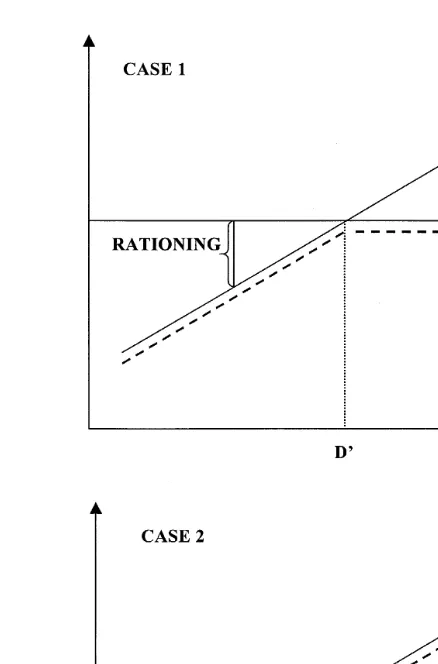
We are now ready to analyse the market for consultations. Fig. 1 shows demand per patient for consultations and supply per patient for consultations as functions of physician density. The broken line represents the market outcome cM.
We define rationing of consultations as a situation where cM-cD and SID as a
( )
[image:5.595.107.326.46.378.2]F. Carlsen, J. GryttenrJournal of Health Economics 19 2000 731–753 735
Fig. 1. The market for consultations.
Ž .
Suppose first Case 1 that patients have complete information about their utility function. Then, the short side of the market determines quantity: cMscD if
D)DX; cMscS if D-DX
. Hence, we have rationing in physician-scarce munici-palities and neither rationing nor SID in physician-dense municimunici-palities. The threshold DX does not depend on the preference parameter l; the weight that contract physicians place on patient utility affects the amount of rationing in physician-scarce municipalities but not whether rationing takes place.1
Ž .
Suppose next Case 2 that patients do not know the utility of consultations, and that the market outcome is determined by the contract physicians: cMscS. Compared to Case 1, the outcome does not change in physician-scarce
( )
F. Carlsen, J. GryttenrJournal of Health Economics 19 2000 731–753
736
ties; we still have rationing and the amount of rationing depends on the physician preference parameter. In physician-dense municipalities, we now have SID. In these municipalities, the extent to which contract physicians care about their patients has no effect on whether SID takes place, but affects the amount of inducement; the more contract physicians care about patient utility, the lower is
Ž M D.
the amount of inducement c yc .
Consider now the policy-maker’s decision problem. In order for policy-makers to be able to compute the physician density which maximizes social welfare for a given fee structure, they need to have information about demand and supply functions. In practice, policy-makers have limited information about the parame-ters of the model; as mentioned in the introduction, there is not even agreement about whether SID exists at all. However, if we accept the assumption that surveys provide information about patient utility, then the policy-maker can use surveys to examine whether physician density is too high or too low.
Suppose that the social welfare function is equal to the utility of a representa-tive patient minus the cost of state expenditure per patient, and that consultations are determined by the physicians. Then the policy-maker prefers the physician density which maximizes:
U
Ž
ycSŽ .
D ,cSŽ .
D.
ygpScSŽ .
Dwhereg is the marginal cost of public funds;g captures the deadweight loss of taxes as well as administrative costs. The first-order condition can be written as:
S S S
Uc
Ž
Ec rED.
s UIqgpŽ
Ec rED ..
Ž .
4Ž . Ž .
The right-hand side of Eq. 4 is the total privateqpublic marginal cost of physician density and can be computed from aggregate data on consultations and
Ž .
other primary care services provided g is known . The left-hand side is the marginal patient utility of physician density and can be computed from surveys provided that reported satisfaction is a valid proxy for patient utility. Thus, even with limited information about the market for primary physician services, includ-ing whether SID takes place, the policy-maker can use surveys to examine whether the marginal utility of physician density is higher or lower than the marginal cost of physician density and thus whether physician density is above or below the social optimum.
3. Data and empirical specification
( )
F. Carlsen, J. GryttenrJournal of Health Economics 19 2000 731–753 737
physician services. For the years 1993–1997, 72,186 respondents returned the questionnaire. We excluded individuals from municipalities with only employed physicians, individuals who did not answer all questions about personal
character-Ž .
istics age, gender, etc. and individuals who belonged to municipalities where characteristics of the municipal population was missing. This left us with a sample of 55,549 individuals. The response rates for the questions on primary physician
Ž .
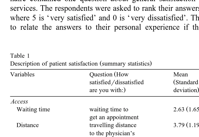
services were in the range 49–72% Table 1 .
[image:7.595.48.390.318.553.2]Since patient fees are regulated by the state, there are two potential ways that physician density can affect consumer satisfaction. First, more physicians may imply better access to care through lower waiting time and lower travelling costs. The questionnaire contained two questions about access to care. The exact wording of the questions is given in Table 1. Secondly, more physicians may imply better quality of care because physicians are able to pay more attention to the problems of each patient, including spending more time with the patient. The questionnaire contained four questions about quality of care. Finally, the question-naire contained one question about general satisfaction with primary physician services. The respondents were asked to rank their answers on a scale from 0 to 5, where 5 is ‘ very satisfied’ and 0 is ‘ very dissatisfied’. The respondents were told to relate the answers to their personal experience if they had seen a primary
Table 1
Ž .
Description of patient satisfaction summary statistics
Ž
Variables Question How Mean Number of
Ž
satisfiedrdissatisfied Standard respondents
. .
are you with: deviation
Access
Ž .
Waiting time waiting time to 2.63 1.65 38,110
get an appointment
Ž .
Distance travelling distance 3.79 1.19 35,472
to the physician’s office
Quality
Ž .
Communication information about 3.60 1.25 27,022
diagnoses and treatment
Ž .
Friendliness the way you were 3.70 1.26 35,016
received at the office
Ž .
Professional skills the physician’s 3.88 1.05 37,467 professional skills
Ž .
Outcome the outcome 3.66 1.21 33,588
of treatment General satisfaction
Ž .
General satisfaction the primary 3.59 1.26 40,006
( )
F. Carlsen, J. GryttenrJournal of Health Economics 19 2000 731–753
738
physician recently. If they had not seen a primary physician recently, they were told to report their general impression of the primary physician services within their municipality.
As the respondents’ answers are ordered discrete numbers, we estimated the following ordered probit model for each dependent variable:
SAT)sPERS b qb DENS qMUN b q´ q´ ,
ji t ji t 1 2 i t i t 3 i t ji t
SAT s0 if SAT)Fm ,
ji t ji t 1
SAT s1 ifm GSAT))m ,
ji t 2 ji t 1
SAT s5 if SAT))m
ji t ji t 5
where SATji t is the evaluation of respondent j in municipality i and year t,
PERSji t is a vector of personal characteristics, DENSi t is physician density in municipality i and year t, and MUNi t is a vector of municipality characteristics other than physician density which may affect demand for and supply of primary physician services. The error terms, ´i t and ´ji t, are assumed to be independent and normally distributed with constant variance;´i t captures random disturbances common to all respondents in municipality i and year t. The ms are unknown parameters to be estimated with the bs. We used LIMDEP 7.0 to estimate the ordered probit model. Due to software limitations, the municipal error term, ´i t, was set to zero when the model was estimated on the full data set or large
Ž .
subsamples Tables 3–5 . The ordered probit model with municipal error term was
Ž .
estimated for a smaller subsample Table 6 .
Table 2 presents variable definitions and summary statistics of the explanatory variables. The personal characteristics include dummy variables for age, gender, marital status, education, and family income. Physician density was defined as primary physician person years per 10,000 inhabitants. The other municipal characteristics were similar to control variables included in earlier studies of
Ž .
()
F.
Carlsen,
J.
Grytten
r
Journal
of
Health
Economics
19
2000
731
–
753
[image:9.595.79.620.71.369.2]739
Table 2
Independent variables
Independent variables Definition Mean
ŽStandard deviation.
Variables at the leÕel of the indiÕidual
Respondent’s age 1 1 if the respondent’s age is between 30 0.61
Ž .
and 59 years Reference category:-30 years
Respondent’s age 2 1 if the respondent’s age isG60 years 0.21
ŽReference category:-30 years.
Respondent’s gender 1 if male 0.51
Respondent’s marital status 1 if married 0.71
Respondent’s level of education 1 1 if the respondent’s highest level of education 0.47
Ž .
is high school Reference category: primary education
Respondent’s level of education 2 1 if the respondent’s highest level of education 0.30
Ž .
is college or university Reference category: primary education
Ž .
Respondent’s family income 1 if respondent’s family incomeGNOK 300,000 £25,000 0.56
Variables at the leÕel of the municipality
Ž .
Physician density Primary care physician person years per 10,000 inhabitants 7.87 1.91
Ž .
Other personnel Person years of other personnel categories in 16.59 7.04
primary health care per 10,000 inhabitants
Ž .
Care for the elderly Input of person years in care for the elderly 0.10 0.03
per inhabitant above 67
Dummy for hospital 0.18
Ž .
Proportion of employed physicians Employed physician person years scaled 0.26 0.26
by primary care physician person years
Ž .
Population Population size 13,047 33,904
Dummy for town 1 if town with more than 10,000 inhabitants 0.28
within 30 min driving
Dummy for Northern Norway 1 if municipality located in Nord-Trøndelag, 0.12
Nordland, Troms or Finnmark
Ž . Ž .
Travelling time Mean travelling time to municipality centre in min 12.84 8.81
Ž .
Mortality Mean number of annual deaths per 100,000 913.8 111.3
inhabitants during 1990 – 1995, adjusted for variation in age composition
Ž .
Welfare clients Number of welfare clients scaled by population above 15 0.04 0.01
Ž .
Education Number of inhabitants with completed colleger 0.10 0.03
()
F.
Carlsen,
J.
Grytten
r
Journal
of
Health
Economics
19
2000
731
–
753
[image:10.842.84.594.131.380.2]740
Table 3
2 Ž .
Determinants of satisfaction with primary physician services. Ordered probit regression. Wald x test statistics absolute values below the regression coefficient
The second column for each dependent variable includes only explanatory variables which are significant at p-0.05.
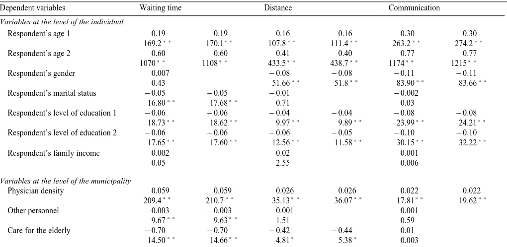
Dependent variables Waiting time Distance Communication
Variables at the leÕel of the indiÕidual
Respondent’s age 1 0.19 0.19 0.16 0.16 0.30 0.30
) ) ) ) ) ) ) ) ) ) ) )
169.2 170.1 107.8 111.4 263.2 274.2
Respondent’s age 2 0.60 0.60 0.41 0.40 0.77 0.77
) ) ) ) ) ) ) ) ) ) ) )
1070 1108 433.5 438.7 1174 1215
Respondent’s gender 0.007 y0.08 y0.08 y0.11 y0.11
) ) ) ) ) ) ) )
0.43 51.66 51.8 83.90 83.66
Respondent’s marital status y0.05 y0.05 y0.01 y0.002
) ) ) )
16.80 17.68 0.71 0.03
Respondent’s level of education 1 y0.06 y0.06 y0.04 y0.04 y0.08 y0.08
) ) ) ) ) ) ) ) ) ) ) )
18.73 18.62 9.97 9.89 23.99 24.21
Respondent’s level of education 2 y0.06 y0.06 y0.06 y0.05 y0.10 y0.10
) ) ) ) ) ) ) ) ) ) ) )
17.65 17.60 12.56 11.58 30.15 32.22
Respondent’s family income 0.002 0.02 0.001
0.05 2.55 0.006
Variables at the leÕel of the municipality
Physician density 0.059 0.059 0.026 0.026 0.022 0.022
) ) ) ) ) ) ) ) ) ) ) )
209.4 210.7 35.13 36.07 17.81 19.62
Other personnel y0.003 y0.003 0.001 0.001
) ) ) )
9.67 9.63 1.51 0.59
Care for the elderly y0.70 y0.70 y0.42 y0.44 0.01
) ) ) ) ) )
()
F.
Carlsen,
J.
Grytten
r
Journal
of
Health
Economics
19
2000
731
–
753
741
Dummy for hospital 0.11 0.11 0.03 0.04 0.10 0.10
) ) ) ) ) ) ) ) ) ) )
62.74 65.36 5.91 8.27 32.46 38.16
Proportion of employed physicians y0.21 y0.21 y0.04 y0.17 y0.17
) ) ) ) ) ) ) )
59.37 59.53 2.31 24.54 28.17
y7 y7 y7 y7 y7 y7
Population 5.60=10 5.60=10 3.45=10 3.68=10 y1.71=10 y1.69=10
) ) ) ) ) ) ) ) ) )
69.60 69.63 23.57 31.43 4.67 6.55
Dummy for town 0.11 0.11 0.08 0.08 0.09 0.09
) ) ) ) ) ) ) ) ) ) ) )
68.40 68.77 32.46 36.14 26.17 34.36
Dummy for Northern Norway y0.17 y0.17 0.06 0.06 y0.03
) ) ) ) ) ) ) )
91.66 91.92 13.05 14.40 1.91
Travelling time y0.002 y0.002 y0.01 y0.01 y0.005 y0.005
) ) ) ) ) ) ) ) ) ) ) )
12.47 12.50 189.7 201.6 41.02 45.06
Mortality y0.0008 y0.0008 y0.0004 y0.0003 y0.0005 y0.0005
) ) ) ) ) ) ) ) ) ) ) )
114.4 115.1 27.22 25.22 33.06 41.20
Welfare clients 1.55 1.55 0.75 2.66 2.70
) ) ) ) ) ) ) )
8.65 8.69 1.74 15.71 19.10
Education y0.83 y0.84 y0.98 y0.98 y0.09
) ) ) ) ) ) ) )
23.30 24.97 28.88 31.61 0.20
Ž .
Mu 1 y0.84 y0.84 0.09 0.11 y0.66 y0.66
129.9 129.8 1.25 2.16 50.10 60.21
Ž .
Mu 2 y0.14 y0.14 0.96 0.99 0.26 0.26
3.80 3.64 144.0 168.6 8.14 9.74
Ž .
Mu 3 0.35 0.35 1.63 1.66 0.94 0.94
22.76 23.39 409.7 470.8 102.6 122.9
Ž .
Mu 4 0.78 0.78 2.18 2.20 1.49 1.49
112.1 114.0 718.9 819.7 255.7 306.2
Ž .
Mu 5 1.32 1.32 2.65 2.68 2.00 2.00
317.1 321.0 1044 1183 450.9 538.4
Concordant 0.60 0.60 0.58 0.58 0.61 0.61
)
p-0.05.
) )
()
F.
Carlsen,
J.
Grytten
r
Journal
of
Health
Economics
19
2000
731
–
753
742
Friendliness Professional skills Outcome General satisfaction
0.25 0.25 0.22 0.22 0.16 0.17 0.26 0.26
) ) ) ) ) ) ) ) ) ) ) ) ) ) ) )
255.0 254.6 209.7 227.0 105.0 114.3 316.4 333.2
0.73 0.73 0.66 0.67 0.59 0.59 0.84 0.84
) ) ) ) ) ) ) ) ) ) ) ) ) ) ) )
1353 1399 1173 1220 866.2 892.9 2070 2132
y0.12 y0.12 y0.18 y0.18 y0.14 y0.14 y0.20 y0.20
) ) ) ) ) ) ) ) ) ) ) ) ) ) ) )
109.9 112.4 282.7 283.1 149.7 148.3 364.6 366.1
y0.01 0.01 0.004 0.002
0.71 1.98 0.11 0.03
y0.10 y0.10 y0.10 y0.10 y0.07 y0.07 y0.15 y0.15
) ) ) ) ) ) ) ) ) ) ) ) ) ) ) )
45.53 46.96 52.20 50.65 25.52 24.52 111.9 111.0
y0.15 y0.16 y0.20 y0.19 y0.14 y0.13 y0.22 y0.22
) ) ) ) ) ) ) ) ) ) ) ) ) ) ) )
85.99 97.02 141.5 140.2 67.53 64.61 201.3 201.2
y0.01 y0.03 y0.02 0.01 y0.02 y0.02
) ) ) ) )
1.13 7.28 5.34 2.24 6.02 5.98
0.030 0.030 0.026 0.026 0.017 0.017 0.035 0.035
) ) ) ) ) ) ) ) ) ) ) ) ) ) ) )
45.77 48.12 39.04 40.10 15.44 15.79 74.75 76.53
0.001 y0.0007 0.0002 y0.0003
0.76 0.57 0.02 0.11
y0.01 0.07 0.14 y0.49 y0.49
) ) ) )
()
F.
Carlsen,
J.
Grytten
r
Journal
of
Health
Economics
19
2000
731
–
753
743
0.08 0.07 0.09 0.09 0.08 0.09 0.08 0.08
) ) ) ) ) ) ) ) ) ) ) ) ) ) ) )
27.66 29.21 40.25 47.54 31.26 39.50 37.90 35.58
y0.21 y0.20 y0.19 y0.21 y0.11 y0.11 y0.21 y0.23
) ) ) ) ) ) ) ) ) ) ) ) ) ) ) )
47.49 49.93 43.28 58.19 13.48 15.27 56.61 74.00
y7 y7 y8 y8 y8
y2.09=10 y2.19=10 y8.79=10 y8.47=10 y7.72=10
) ) ) )
8.69 13.00 1.58 1.38 1.32
0.10 0.10 0.11 0.11 0.09 0.09 0.12 0.13
) ) ) ) ) ) ) ) ) ) ) ) ) ) ) )
48.43 58.39 55.52 82.89 39.07 51.52 79.75 88.90
y0.03 y0.03 y0.04 y0.03 y0.03
) )
2.59 2.93 5.64 4.23 3.57
y0.005 y0.005 y0.005 y0.006 y0.006 y0.006 y0.004 y0.005
) ) ) ) ) ) ) ) ) ) ) ) ) ) ) )
50.66 58.48 47.52 60.75 50.07 62.21 38.62 47.77
y0.0005 y0.0005 y0.0004 y0.0003 y0.0004 y0.0003 y0.0007 y0.0007
) ) ) ) ) ) ) ) ) ) ) ) ) ) ) )
40.00 43.98 28.74 30.84 24.34 22.70 93.06 95.08
1.71 1.85 1.03 1.15 2.42 2.12
) ) ) ) ) ) ) )
8.91 11.75 3.61 3.91 21.12 19.16
y0.15 y0.37 y0.50 y0.41 y0.48 y0.85 y0.93
) ) ) ) ) ) ) ) ) )
0.68 4.21 12.49 4.83 10.62 24.76 39.59
y0.32 y0.35 y0.35 y0.34 y0.32 y0.28 y0.10 y0.07
15.64 24.45 21.70 23.56 15.77 15.25 2.19 1.09
0.57 0.53 0.69 0.70 0.63 0.67 0.77 0.81
49.93 54.86 82.50 99.18 60.08 83.91 110.6 139.7
1.20 1.16 1.49 1.50 1.37 1.40 1.49 1.52
220.6 260.2 378.5 446.4 277.1 363.3 406.7 490.6
1.71 1.67 2.06 2.07 1.86 1.90 2.06 2.09
443.3 531.6 708.1 829.5 509.8 657.4 771.5 917.0
2.17 2.13 2.49 2.50 2.30 2.34 2.55 2.58
701.8 847.2 1007 1172 764.1 974.2 1161 1367
( )
F. Carlsen, J. GryttenrJournal of Health Economics 19 2000 731–753
[image:14.595.48.384.98.284.2]744 Table 4
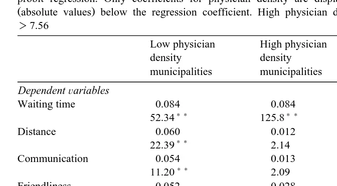
Impact of physician density on satisfaction in lowrhigh physician density municipalities. Ordered probit regression. Only coefficients for physician density are displayed. Wald x2 test statistics Žabsolute values below the regression coefficient. High physician density area: Physician density.
)7.56
2 Low physician High physician Waldx
a
density density test statistics
municipalities municipalities
DependentÕariables
Waiting time 0.084 0.084 0.20
) ) ) )
52.34 125.8
) )
Distance 0.060 0.012 12.03
) )
22.39 2.14
)
Communication 0.054 0.013 6.30
) )
11.20 2.09
Friendliness 0.052 0.028 1.25
) ) ) )
17.20 12.09
Professional skills 0.039 0.025 0.67
) ) ) )
10.86 11.04
Outcome 0.036 0.009 1.70
) )
7.76 1.17
) )
General satisfaction 0.072 0.036 7.19
) ) ) )
38.58 22.93
aWald x2 test statistics absolute values refer to the interaction term between physician densityŽ . and a dummy variable for high physician density municipalities in pooled regressions.
)
p-0.05.
) )
p-0.01.
Second, the control variables measured demographic characteristics of the municipalities which may affect accessibility to primary physician services. The following variables were included: population size, dummies for town and North-ern Norway, and the mean travelling time to the municipality centre. Third, the control variables measured the health status of the population. The following variables were included: mortality rate, proportion of welfare clients and average education level. All variables at the level of the municipality were obtained from the Norwegian Social Science Data Service.
4. Results and discussion
()
F.
Carlsen,
J.
Grytten
r
Journal
of
Health
Economics
19
2000
731
–
753
[image:15.595.89.598.81.354.2]745
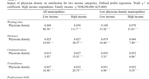
Table 5
2 Ž .
Impact of physician density on satisfaction for two income categories. Ordered probit regression. Wald x test statistics absolute values below the regression
Ž .
coefficient. High income respondents: Family income GNOK300,000 £25,000
All municipalities Low physician density municipalities High physician density municipalities Low income High income Low income High income Low income High income
Waiting time
Physician density 0.060 0.058 0.100 0.070 0.079 0.089
) ) ) ) ) ) ) ) ) ) ) )
98.38 111.7 31.92 21.01 51.69 75.02
Distance
Physician density 0.025 0.027 0.079 0.046 0.007 0.017
) ) ) ) ) ) ) )
14.84 20.57 16.44 7.49 0.35 2.57
Communication
Physician density 0.015 0.027 0.058 0.052 0.006 0.019
) ) ) ) )
3.85 15.81 5.31 6.06 0.25 2.62
Friendliness
Physician density 0.027 0.032 0.051 0.052 0.038 0.022
) ) ) ) ) ) ) ) ) ) )
16.98 29.75 6.94 9.55 9.98 4.15
Professional skills
Physician density 0.027 0.026 0.037 0.039 0.035 0.019
) ) ) ) ) ) ) )
18.43 20.75 4.17 6.16 9.81 3.39
Outcome
Physician density 0.017 0.017 0.021 0.045 0.018 0.0009
) ) ) ) ) )
7.05 8.34 1.13 6.94 2.28 0.006
General satisfaction
Physician density 0.023 0.046 0.049 0.088 0.030 0.044
) ) ) ) ) ) ) ) ) ) ) )
13.94 69.95 7.35 33.55 7.44 18.46
()
F.
Carlsen,
J.
Grytten
r
Journal
of
Health
Economics
19
2000
731
–
753
[image:16.842.90.597.153.379.2]746
Table 6
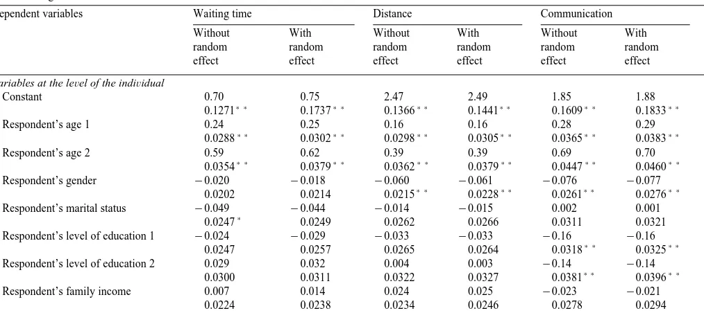
Ž .
Determinants of satisfaction with primary physician services. Ordered probit regression with and without random effects. Standard error absolute values below the regression coefficient
Dependent variables Waiting time Distance Communication
Without With Without With Without With
random random random random random random
effect effect effect effect effect effect
Variables at the leÕel of the indiÕidual
Constant 0.70 0.75 2.47 2.49 1.85 1.88
) ) ) ) ) ) ) ) ) ) ) )
0.1271 0.1737 0.1366 0.1441 0.1609 0.1833
Respondent’s age 1 0.24 0.25 0.16 0.16 0.28 0.29
) ) ) ) ) ) ) ) ) ) ) )
0.0288 0.0302 0.0298 0.0305 0.0365 0.0383
Respondent’s age 2 0.59 0.62 0.39 0.39 0.69 0.70
) ) ) ) ) ) ) ) ) ) ) )
0.0354 0.0379 0.0362 0.0379 0.0447 0.0460
Respondent’s gender y0.020 y0.018 y0.060 y0.061 y0.076 y0.077
) ) ) ) ) ) ) )
0.0202 0.0214 0.0215 0.0228 0.0261 0.0276
Respondent’s marital status y0.049 y0.044 y0.014 y0.015 0.002 0.001
)
0.0247 0.0249 0.0262 0.0266 0.0311 0.0321
Respondent’s level of education 1 y0.024 y0.029 y0.033 y0.033 y0.16 y0.16
) ) ) )
0.0247 0.0257 0.0265 0.0264 0.0318 0.0325
Respondent’s level of education 2 0.029 0.032 0.004 0.003 y0.14 y0.14
) ) ) )
0.0300 0.0311 0.0322 0.0327 0.0381 0.0396
Respondent’s family income 0.007 0.014 0.024 0.025 y0.023 y0.021
()
F.
Carlsen,
J.
Grytten
r
Journal
of
Health
Economics
19
2000
731
–
753
747
Variables at the leÕel of the municipality
Physician density 0.059 0.061 0.022 0.022 0.024 0.024
) ) ) ) ) ) ) ) ) ) ) )
0.0057 0.0078 0.0058 0.0062 0.0070 0.0080
Other personnel y0.003 y0.003 0.002 0.002 y0.0001 y0.0001
0.0014 0.0021 0.0015 0.0014 0.0019 0.0029
Care for the elderly 0.58 0.67 0.28 0.29 0.30 0.27
0.4219 0.5891 0.4451 0.4593 0.5230 0.5980
Dummy for hospital 0.078 0.077 0.074 0.074 0.12 0.12
) ) ) ) ) ) ) )
0.0281 0.0433 0.0297 0.0332 0.0380 0.0416
Proportion of employed physicians y0.20 y0.21 y0.055 y0.055 y0.13 y0.13
) ) ) ) ) ) )
0.0404 0.0554 0.0424 0.0435 0.0515 0.0602
y5 y5 y7 y7 y6 y6
Population 0.10=10 0.11=10 y0.11=10 y0.10=10 y0.41=10 y0.42=10
y6) ) y6 y6 y6 y6 y6
0.30=10 0.56=10 0.35=10 0.37=10 0.45=10 0.46=10
Dummy for town 0.033 0.030 0.077 0.78 0.053 0.054
) ) ) )
0.0267 0.0433 0.0278 0.0290 0.0340 0.0376
Dummy for Northern Norway y0.29 y0.30 0.037 0.037 y0.060 y0.060
) ) ) )
0.0324 0.0475 0.0346 0.0391 0.0412 0.0469
Travelling time y0.001 y0.001 y0.011 y0.011 y0.003 y0.003
) ) ) )
0.0013 0.0018 0.0013 0.0012 0.0015 0.0019
Mortality y0.0002 y0.0002 y0.0003 y0.0003 y0.0004 y0.0004
) ) ) ) ) )
0.0001 0.0001 0.0001 0.0001 0.0001 0.0002
Welfare clients y1.99 y2.14 y2.65 y2.68 1.25 1.24
) ) ) ) )
0.8693 1.2255 0.9168 0.9722 1.1243 1.2530
Education y0.18 y0.25 y0.10 y0.097 1.06 1.07
) )
0.3809 0.5734 0.4036 0.4242 0.4895 0.5231
)
p-0.05.
) )
()
F.
Carlsen,
J.
Grytten
r
Journal
of
Health
Economics
19
2000
731
–
753
748
Friendliness Professional skills Outcome General satisfaction
Without With Without With Without With Without With
random random random random random random random random
effect effect effect effect effect effect effect effect
1.88 1.89 2.37 2.41 2.28 2.30 2.16 2.20
) ) ) ) ) ) ) ) ) ) ) ) ) ) ) )
0.1346 0.1501 0.1444 0.1672 0.1341 0.1461 0.1300 0.1438
0.23 0.24 0.22 0.23 0.17 0.17 0.25 0.26
) ) ) ) ) ) ) ) ) ) ) ) ) ) ) )
0.0293 0.0290 0.0308 0.0324 0.0298 0.0318 0.0284 0.0289
0.70 0.71 0.67 0.70 0.57 0.57 0.77 0.78
) ) ) ) ) ) ) ) ) ) ) ) ) ) ) )
0.0363 0.0369 0.0394 0.0411 0.0366 0.0383 0.0357 0.0358
y0.096 y0.097 y0.17 y0.18 y0.16 y0.16 y0.21 y0.21
) ) ) ) ) ) ) ) ) ) ) ) ) ) ) )
0.0214 0.0217 0.0228 0.0236 0.0214 0.0220 0.0206 0.0213
0.009 0.009 0.010 0.010 0.022 0.023 0.016 0.019
0.0256 0.0257 0.0277 0.0284 0.0255 0.0257 0.0253 0.0258
y0.11 y0.11 y0.12 y0.13 y0.067 y0.066 y0.18 y0.19
) ) ) ) ) ) ) ) ) ) ) ) ) ) )
0.0261 0.0260 0.0280 0.0282 0.0258 0.0259 0.0255 0.0256
y0.15 y0.15 y0.18 y0.18 y0.11 y0.11 y0.21 y0.22
) ) ) ) ) ) ) ) ) ) ) ) ) ) ) )
0.0320 0.0324 0.0341 0.0341 0.0320 0.0321 0.0309 0.0316
y0.007 y0.007 y0.036 y0.032 0.001 0.001 y0.068 y0.071
) ) ) )
()
F.
Carlsen,
J.
Grytten
r
Journal
of
Health
Economics
19
2000
731
–
753
749
0.028 0.028 0.030 0.030 0.012 0.012 0.028 0.029
) ) ) ) ) ) ) ) ) ) ) ) )
0.0060 0.0065 0.0061 0.0067 0.0059 0.0060 0.0056 0.0061
0.0004 0.0005 0.002 0.002 0.001 0.001 0.0001 0.0001
0.0016 0.0017 0.0016 0.0022 0.0016 0.0022 0.0015 0.0016
0.058 0.038 0.25 0.23 y0.71 y0.72 0.54 0.52
0.4446 0.4808 0.4678 0.5221 0.4422 0.4928 0.4288 0.4593
0.062 0.063 0.071 0.072 0.10 0.10 0.12 0.12
) ) ) ) ) ) ) ) ) )
0.0291 0.0313 0.0326 0.0393 0.0293 0.0314 0.0287 0.0351
y0.13 y0.13 y0.17 y0.17 y0.068 y0.068 y0.17 y0.17
) ) ) ) ) ) ) ) ) ) ) )
0.0432 0.0474 0.0452 0.0539 0.0430 0.0469 0.0408 0.0459
y6 y6 y6 y6 y7 y7 y6 y6
y0.10=10 y0.11=10 0.11=10 0.10=10 y0.34=10 y0.36=10 y0.28=10 y0.29=10
y6 y6 y6 y6 y6 y6 y6 y6
0.31=10 0.52=10 0.35=10 0.41=10 0.34=10 0.41=10 0.32=10 0.39=10
0.058 0.058 0.087 0.087 0.056 0.057 0.066 0.067
) ) ) ) ) ) )
0.0278 0.0307 0.0301 0.0355 0.0278 0.0296 0.0265 0.0303
y0.049 y0.049 y0.026 y0.028 y0.061 y0.061 y0.075 y0.077
) )
0.0342 0.0358 0.0372 0.0427 0.0345 0.0350 0.0329 0.0354
y0.004 y0.004 y0.004 y0.005 y0.003 y0.003 y0.003 y0.003
) ) ) ) ) ) ) ) ) ) ) )
0.0013 0.0015 0.0015 0.0017 0.0014 0.0016 0.0013 0.0014
y0.0002 y0.0002 y0.0004 y0.0004 y0.0002 y0.0002 y0.0002 y0.0002
) ) ) ) ) )
0.0002 0.0001 0.0001 0.0001 0.0001 0.0001 0.0001 0.0001
0.37 0.36 y2.29 y2.31 y0.53 y0.57 y1.62 y1.70
) )
0.9314 0.9929 0.9834 1.1186 0.9318 1.0298 0.8913 1.0149
0.32 0.34 0.70 0.74 y0.078 y0.071 y0.14 y0.12
( )
F. Carlsen, J. GryttenrJournal of Health Economics 19 2000 731–753
750
find that consumers are most satisfied with physician competence and the outcome Ž
of care, and least satisfied with access to care for a review see: Hall and Dornan, .
1988 .
Table 3 presents regressions based on the full data set. Two regressions are presented for each dependent variable. In the first column, all explanatory
Ž .
variables are included, whereas only statistically significant variables p-0.05 are included in the second column. The two specifications produced virtually identical coefficients.
Ž .
Consistent with US surveys Pascoe, 1983; Cleary and McNeil, 1988 , we found that older people, women, and less educated people were more satisfied than younger people, men and people with higher education. There was also some indication that married people and people with high income were relatively dissatisfied with primary physician services.
Physician density was positively associated with all aspects of satisfaction, and the coefficient was always statistically significant at conventional levels of
signifi-Ž .
cance p-0.05 . The impact of physician density on reported satisfaction was strongest for waiting time and weakest for outcome of care and communication. The results thus indicate that physician density is more important for access to care than for quality of care. In general, the coefficients of the other municipal variables are plausible: people were more satisfied with primary physician services in towns, municipalities with a hospital, densely populated municipalities and municipalities with low mortality.
To examine whether the relationship between reported satisfaction and physi-cian density is non-linear, we split the sample into low density and high density municipalities and replicated the parsimonious regressions reported in Table 3 for each subsample.2 The results reported in Table 4 suggest that the impact of
physician density on satisfaction is a decreasing function of physician density. For six of the dependent variables, the coefficient of physician density was higher in the low density sample than in the high density sample, and the difference between the subsamples was statistically significant for three of these six variables. The coefficient of physician density was always significant in the low density sample but only significant for four out of seven dependent variables in the high density sample.
Satisfaction with waiting time to get an appointment was the exception; the coefficient of physician density was equal in the two subsamples. This result suggests that diminishing return to physician density sets in at a higher level of physician density for waiting time than for the other dependent variables. One possible reason is that people on average are less satisfied with waiting time than
Ž .
with the other aspects of primary physician services Table 1 .
2
( )
F. Carlsen, J. GryttenrJournal of Health Economics 19 2000 731–753 751
We expect policy-makers to be particularly interested in the relationship between supply of primary physician services, and access to and quality of care for low income groups. Table 5 presents separate analyses for high and low income respondents using family income as split criterion.3 The results suggest that there are no systematic differences between the two groups.
Finally, we constructed a small subsample by drawing five respondents from each municipality and year. We estimated the ordered probit model on this subsample both with and without the municipal error term to check whether the results presented in Tables 3–5 were biased when the municipal error term was excluded. The results reported in Table 6 suggest that this is not the case; inclusion of the municipal error term has only a modest impact on the coefficients and the estimated standard deviations of the coefficients.
5. Conclusion
We have presented an empirical analysis which shows that citizens are more satisfied with primary physician services the higher the number of primary physicians relative to the population becomes. For most dimensions of satisfaction, there are diminishing returns to physicians; the impact of physician density on reported satisfaction is a decreasing function of physician density. Referring back to the theoretical framework, and bearing in mind that the analyses rest on the assumption that reported satisfaction is a valid proxy for patient utility, these results suggest that a socially optimal density of physicians exists where the marginal benefits of physicians in terms of higher consumer satisfaction are equal
Ž .
to the total privateqpublic marginal costs of physicians. The socially optimal physician density as defined in the paper is conditional on the fee structure and depends on the money value of improved satisfaction as well as on a range of municipal characteristics, but can be computed without knowledge about whether SID exists. We neither attempted to estimate the socially optimal physician density for Norwegian municipalities nor to characterize the optimal fee structure. These challenges are left for future work.
In the present study, we have used perceived measures of satisfaction with primary physician services, rather than objective indicators of health status to assess the impact of physician density. Our output measures are similar to those
Ž .
suggested by Mooney et al. 1991 . They argue that equity in health care should be measured in terms of access, rather than in terms of utilization and improvements in health. Our results indicate that local governments can influence the level of satisfaction with primary physician services by determining the level of supply. However, our results do not say anything about the relationship between supply of
3
( )
F. Carlsen, J. GryttenrJournal of Health Economics 19 2000 731–753
752
services and health status. This is a limitation of our study, as policy-makers are likely to be concerned about whether the extra money spent on improving access leads to better health.
Acknowledgements
We wish to thank Irene Skau and Erik Lund for valuable technical assistance, and Linda Grytten for correcting the language. Finally, thanks for financial support from the Ministry of Health and Social Affairs.
References
Berkanovic, E., Marcus, A., 1976. Satisfaction with health services: some policy implications. Medical Care 14, 873–878.
Carlsen, F., Grytten, J., 1998. More physicians: improved availability or induced demand? Health Economics 7, 495–508.
Cleary, P., McNeil, B., 1988. Patient satisfaction as an indicator of quality care. Inquiry 25, 25–36. Cromwell, J., Mitchell, J., 1986. Physician-induced demand for surgery. Journal of Health Economics
5, 293–313.
Dranove, D., Wehner, P., 1994. Physician-induced demand for childbirths. Journal of Health Eco-nomics 13, 61–73.
Ž .
Feldman, R., Sloan, F., 1988. Competition among physicians, revisited. In: Greenberg, W. Ed. , Competition in the Health Care Sector: Ten Years Later. Duke Univ. Press.
Fuchs, V., 1978. The supply of surgeons and the demand for operations. Journal of Human Resources 13, 35–56.
Grytten, J., Carlsen, F., Sørensen, R., 1995. Supplier inducement in a public health care. Journal of Health Economics 14, 207–229.
Hall, J., Dornan, M., 1988. What patients like about their medical care and how often they are asked: a meta-analysis of the satisfaction literature. Social Science and Medicine 27, 935–939.
Kincey, J., Bradshaw, P., Ley, P., 1975. Patients’ satisfaction and reported acceptance of advice in general practice. Journal of the Royal College of General Practitioners 25, 558–566.
Labelle, R., Stoddard, G., Rice, T., 1994. A re-examination of the meaning and importance of supplier-induced demand. Journal of Health Economics 13, 347–368.
Linn, M., Linn, B., Stein, S., 1982. Satisfaction with ambulatory care and compliance in older patients. Medical Care 20, 606–614.
Marquis, S., Davies, A., Ware, J., 1983. Patient satisfaction and change in medical care provider: a longitudinal study. Medical Care 21, 821–829.
Mooney, G., Hall, J., Donaldson, C., Gerard, K., 1991. Utilisation as a measure of equity: weighing heat? Journal of Health Economics 10, 475–480.
Pascoe, G., 1983. Patient satisfaction in primary health care: a literature review and analysis. Evaluation and Program Planning 6, 185–210.
Phelps, C., 1986. Induced demand — can we ever know its extent? Journal of Health Economics 5, 355–365.
( )
F. Carlsen, J. GryttenrJournal of Health Economics 19 2000 731–753 753
Rice, T., Labelle, R., 1989. Do physicians induce demand for medical services? Journal of Health Politics, Policy and Law 14, 587–600.
Rossiter, L., Wilensky, G., 1984. Identification of physician-induced demand. Journal of Human Resources 19, 231–244.
Ryan, M., 1992, The economic theory of agency in health care: lessons from non-economists for
Ž .
economists, Discussion Paper No 03r92 Health Economics Research Unit, Aberdeen .
Stano, M., 1985. An analysis of the evidence on competition in the physician services markets. Journal of Health Economics 4, 197–211.
Statistics Norway, 1996. Inntekts-og kostnadsundersøkelse for privatpraktiserende leger, 1995. Leger med driftstilskuddsavtale har best driftsresultat, Ukens Statistikk 37, 3–4.
Statistics Norway, 1998. Lege, fysioterapi og forebyggjande tenester i kommunehelsetenesta, 1997. Førebels tal, Ukens statistikk 35, 10–11.
Stewart, M.A., 1995. Effective physician–patient communication and health outcomes. Canadian Medical Association 152, 1423–1433.
Tussing, A., 1983. Physician-induced demand for medical care: Irish general practitioners. Economic and Social Review 14, 225–247.