Directory UMM :Journals:Journal of Health Economics:Vol19.Issue5.Sep2000:

www.elsevier.nlrlocatereconbase

Standard errors for the retransformation problem

with heteroscedasticity

Chunrong Ai

a

, Edward C. Norton

b,) a

UniÕersity of Florida, Florida, USA b

Department of Health Policy and Administration, CBa7400, McGaÕran-Greenberg Building, UniÕersity of North Carolina at Chapel Hill, Chapel Hill, NC, 27599-7400, USA

Received 1 September 1999; received in revised form 1 March 2000; accepted 8 March 2000

Abstract

Economists often estimate models with a log-transformed dependent variable. The results from the log-transformed model are often retransformed back to the unlogged scale. Other studies have shown how to obtain consistent estimates on the original scale but have not provided variance equations for those estimates. In this paper, we derive the variance for three estimates — the conditional mean of y, the slope of y, and the average slope of y — on the retransformed scale. We then illustrate our proposed procedures with skewed health expenditure data from a sample of Medicaid eligible patients with severe mental illness.q2000 Elsevier Science B.V. All rights reserved.

JEL classification: C20; I19

Keywords: Retransformation; Heteroscedasticity; Logged dependent variable

1. Introduction

Economists often estimate models with a log-transformed dependent variable. Justifications for using the log transformation include to deal with a dependent variable badly skewed to the right, and to interpret a covariate as either an

Ž .

elasticity or having a multiplicative response Manning, 1998 . The results from

)_{Corresponding author. Tel.:q1-919-966-8930; fax:q1-919-966-6961.}

Ž .

E-mail address: edward norton@unc.edu E.C. Norton ._–

0167-6296r00r$ - see front matterq2000 Elsevier Science B.V. All rights reserved.

Ž .

the log-transformed model are often retransformed back to the unlogged scale to make inferences in the natural units of, say, dollars instead of log dollars. A log-transformed model is often the second part of the two-part model of health

Ž

care expenditures when some individuals have zero expenditure Duan et al.,

.

1983, 1984 .

It is now well known that the retransformed estimate of either the conditional

Ž .

mean or the effect of an independent variable on the dependent variable the slope must adjust for the distribution of the error term and for heteroscedasticity

ŽManning, 1998; Mullahy, 1998 . Failure to account for the distribution of the.

error term and heteroscedasticity may lead to substantially biased estimates of the conditional mean and the slope on the original scale.

Many studies have carefully addressed the retransformation problem by ex-plaining how inferences on the original scale may be biased, providing equations,

Ž

and illustrating with examples e.g. Duan et al., 1983; Manning, 1998; Mullahy,

.

1998 . However, these studies have not fully addressed the standard errors of the estimates. Like any other estimates, the estimates on the original scale of the conditional mean and the slope are calculated with uncertainty. Without computing the correct standard errors, it would be easy to draw incorrect inferences about the effect of an independent variable on the dependent variable. When testing theory on the raw scale, the statistical significance of the corresponding parameter is not always a good guide. An insignificant variable on the log scale can still have a significant effect on the raw scale, for example if there is heteroscedasticity. A significant variable on the log scale, on the other hand, may be insignificant on the raw scale. Significance on the raw scale depends on retransforming both the predicted value and heteroscedasticity, and these two effects may offset each other. Theory on the raw scale must be tested on the raw scale, and to test theory one must have standard errors or confidence intervals. Like the estimates them-selves, the standard errors require special equations that take into account both the distribution of the error term and the heteroscedasticity. We are not aware of any published formulas for computing the standard error of estimates based on the

Ž Ž .

retransformed data see Manning 1998 for estimates of the variance of the

.

expenditure data from a sample of Medicaid eligible patients with severe mental illness. We derive formulas for the log transformation because it is by far the most common in the literature. Researchers should read the literature and investigate the data empirically to decide whether the log transformation is most appropriate for

Ž .

their data Jones and Yen, 1999; Manning and Mullahy, 1999 .

2. Framework and methods

Before deriving the variance formulas for the most general case, we start with the familiar normal linear model for a log-transformed dependent variable. The normal linear model provides intuition for the more general models, and is the model that is most often estimated by applied economists. Then we extend the model to the nonlinear case, which involves only a slight modification, before presenting the nonparametric model. The nonparametric model has the normal

Ž .

linear and nonlinear models as special cases, and we relate it to Duan’s 1983 smearing estimator.

2.1. Model and notation

We start by introducing the general model and notation. Assume that the

Ž .

logarithm of the original dependent variable y is a possibly nonlinear function of

K explanatory variables x, including a constant, and a vector of unknown

Ž .

parameters b. The model for a single observation we suppress the subscript i can be written as

ln y

Ž .

sh x ,

Ž

b

.

q´,

where´ is an additive error term. We assume that no regressor can be expressed as a linear or nonlinear function of the other regressors, e.g. there are no higher-order or interaction terms. This assumption is not as restrictive as it appears since it can always be satisfied by redefining the function h. For example, if x

Ž .

includes a constant, income, and income squared, then the function h x,b can be redefined as a function of a constant and income. The error term ´ is the product of two elements

(

´sy s x ,

Ž

a

.

wherey is assumed to be independent of x and has zero mean and unit variance,

Ž .

We are interested in three estimands based on the unlogged dependent variable

y. The first is the mean of y conditional on x. This is the predicted value of the

Ž

raw dependent variable for one specific x. The second is the derivative local

. k

slope of the mean with respect to one continuous explanatory variable x conditional on x, where xk _{denotes the k th element of x. This is the change in the}

predicted value for a change in one independent variable, for one specific x. The third estimand depends on whether the regressors are treated as nonrandom or random. If the regressors are nonrandom, the third estimand is the simple average slope over all observations. If the regressors are random the third estimand is the average slope over the parent distribution of the regressors.

Ž .

We introduce the notation thatm x is the mean of y conditional on x and that

u1 and u2 denote the two average slopes. This notation will simplify later formulas. The function also depends on the true values of b and a, but these arguments will be suppressed for exposition. The estimands are as follows.

Ø Mean of y conditional on x

w

x

m

Ž .

x sE yNx ,

Ø Slope of mean with respect to xk

w

x

Em

Ž .

x EE yNx

s ,

k k

Ex Ex

Ž .

Ø Average slope two versions

N

1 Em

Ž

xi

.

for nonrandom x :u1s_N

Ý

_Exk .

is1

Em

Ž .

x

for random x :u2sE _E k .

x

2.2. Normal linear model

To present the intuition behind our procedures, we begin with the simple

Ž . X

normal linear model. The assumption of linearity implies that h x,b sxb and

Ž . X

s x,a sxa. Note that because elements of x are functionally independent, the

Ž . Ž .

functions h x,b and s x,a are not only linear in the parameters but also linear in the regressors. This distinction becomes important when taking derivatives. If

Ž . Ž . Ž

either h x,b or s x,a is linear in parameters but nonlinear in regressors e.g.

. k

nonnested models is to use the J-test for linear specifications, and the PE test for

Ž .

nonlinear specifications see Greene, 2000, pp. 302 and 441 .

Consistent estimates for the slope and the average slope for a model nonlinear in the regressors can be obtained using the formulas in Section 2.3. We also assume that the random variable y has a standard normal distribution. The

Ž .

assumption of normality is attractive because: 1 it is often assumed in the

Ž . Ž

literature, and 2 the retransformed estimands are simple to derive Manning,

.

1998, pp. 285–287 .

Under the assumptions of linearity and normality the first two estimands for fixed x are

w

x

xXbq0 .5 xXa

m

Ž .

x sE yNx se ,

Em

Ž .

x

s

Ž

bkq0.5ak

. Ž .

m x ,

k Ex

where the subscript k refers to the k th component of the parameter vector. Estimate the three estimands by replacing b and a with consistent estimates. To estimatea, regress the squared residuals from the ordinary least squares model on

x, then multiply x by the estimated parameter vectora

ˆ

. Then the estimated mean of y conditional on x is the exponentiated predicted value of y, with a correction for the variance of the normal error term

X _ˆ X

x bq0 .5 xaˆ

m

ˆ

Ž .

x se .

The estimated slope with respect to one continuous variable xk _{is the mean}

Ž .

multiplied by the sum of two terms. The following is similar to Manning’s 1998

Ž .

Eq. 7 , but we assume a particular form of the heteroscedasticity, namely

Ž . X

s x,a

ˆ

sxa

ˆ

, so the slope is

Em

ˆ

Ž .

x

ˆ

s

ž

bkq0.5a

ˆ

k

/

m

ˆ

Ž .

x .

k Ex

Finally, both versions of the third estimand are estimated by the sample average of the slope over all observations because the expectation is usually approximated by the sample average, leading to

N

1 Em

ˆ

Ž

xi

.

ˆ

ˆ

u1su2s_N

Ý

_E k .

x

is1

ˆ

many degrees of freedom looks like a normal distribution and so can be approxi-mated by a normal distribution when sample size goes to infinity. Hence, the

ˆ

parameter estimatora

ˆ

is asymptotically normally distributed. Moreover, b and a

ˆ

are independent. Thus, applying the delta method gives the scalar variance of these three estimands

Em

Ž .

x Em

Ž .

x Em

Ž .

x Em

Ž .

x

v1

Ž .

x s

ž

_EbX Sb _Eb

/

q

ž

_EaX Sa _Ea

/

,

Ž .

1

E2m

Ž .

x E2m

Ž .

x E2m

Ž .

x E2m

Ž .

x

v2 k

Ž .

x s

ž

_Exk_EbXSb _EbExk

/

q

ž

_Exk_EaXSa _EaExk

/

,

Ž .

2

N 2 N 2

1 Em

Ž

xi

.

1 Em

Ž

xi

.

v3 ks

ž

ž

_N

Ý

_Exk_EbX

/ ž

Sb _N

Ý

_EbExk

/

/

is1 is1

N 2 N 2

1 Em

Ž

xi

.

1 Em

Ž

xi

.

q

ž

ž

_N

Ý

_Exk_EaX

/ ž

Sa _N

Ý

_EaExk

/

/

,

Ž .

3

is1 is1

2 2

Em

Ž .

x Em

Ž .

x

v4 ks

ž

E _Exk_EbX SbE _EbExk

/

2 2

Em

Ž .

x Em

Ž .

x

q

ž

E _E k X SaE k

/

qSm,

Ž .

4

x Ea EaEx

Ž .

where the terms withEm x in the numerator are first partial derivatives, the terms

2 _{Ž .}

withEm x in the numerator are second partial derivatives, and S_b and S_a are the heteroscedasticity consistent covariance matrices for b and a, respectively.

Ž

The White heteroscedasticity consistent estimator can be found in Greene 2000,

.

p. 463 and can be computed by most regression packages. The third term of Eq.

Ž ._{4 , S , is the sample variance of Em}Ž_x._{rEx divided by N. This term is needed}k

m i

because we use the sample average to estimate the average slope over the parent distribution of the regressors.

Before describing how to estimate these in practice, we first note several features of these variances. Each variance is a scalar. Each variance is the sum of

Ž .

two or three parts; the first part corresponds to the retransformation of the

Ž .

predicted value of ln y , and the second part corresponds to the retransformation of the error term with estimated heteroscedasticity. Each of the first two parts is a sandwich estimator.

In summary, the computation of the estimated variance for the normal linear model requires four steps. Estimate the model on the log scale, estimate the form

Ž .

of heteroscedasticity, compute several derivatives the hardest step , and plug the

Ž . Ž .

Step I: Apply ordinary least squares to the logarithm of y on x . Compute thei i

X

ˆ

scalar predicted value xb for some fixed x. Save the heteroscedasticity-consistent

ˆ

covariance matrix as Sb. Save the residuals ´

ˆ

i, and square them. Step II: Apply ordinary least squares to ´2

on x . Compute the scalar predicted

ˆ

i i

value xXa

ˆ

for some fixed x. Save the heteroscedasticity-consistent covariance

ˆ

matrix as S_a.

Ž . Ž .

Step III: Compute m

ˆ

x , and the first derivatives of m

ˆ

x with respect to b,

Ž a, and x, and their cross partial derivatives either numerically or analytically see

.

Appendix A for formulas . To estimate S_m, compute the sample variance of

Ž . k

am

ˆ

xi rEx .

Ž . Ž .

Step IV: Plug the estimated values from Step III into Eqs. 1 – 4 . The

X

ˆ

X

ˆ

₂

Ž . Ž . Ž . Ž .

equation for v

ˆ

1 x simplifies to v

ˆ

1 x s xSbxq0.25 xSax m

ˆ

x , although

the other equations do not simplify.

2.3. Normal nonlinear model

Next we extend the linear results to nonlinear models but maintain the normality assumption. There are three ways the nonlinear model is a generaliza-tion of the linear model. First, the nonlinear model allows nonlinearity in regressors. In our notation, the linear specification excludes squared and interac-tion terms which are commonly used in the empirical economic literature. Although squared and interaction terms can be estimated using ordinary least squares, such a specification has more complex derivatives than the simple linear model, so is included in this section. Second, the nonlinear model allows for arbitrary nonlinear functions of the dependent variable to be estimated by least

Ž Ž . X

.

squares. Third, the linear specification of the variance of the error s x,a

ˆ

sxa

ˆ

could allow a negative estimate, which is clearly impossible for the variance itself. The nonlinear specification such as exXa

guarantees that the estimated variance will always be positive. In addition one may wish to include higher-order and interaction terms in the variance function.

ˆ

The parameter estimates b and a

ˆ

now can be obtained by nonlinear least

Ž . Ž .

squares regressions, or by ordinary least squares if h x,b and s x,a are linear

ˆ

in the parameters. The parameter estimates b and a

ˆ

are now asymptotically

Ž .

independent and normally distributed see Appendix A for a formal proof . Hence,

Ž . Ž .

Eqs. 1 – 4 are still valid. Despite these changes, the four steps for computing the three estimands and their respective standard errors are nearly the same as before except that the derivatives are more complicated.

Ž .

Step I: Apply nonlinear least squares, or ordinary least squares if h x,b is

Ž .

linear in the parameters, to the logarithm of y on h x ,_{i i} b . Compute the scalar

ˆ

Ž .

predicted value h x,b for some fixed x. Save the heteroscedasticity-consistent

ˆ

covariance matrix as Sb. Save the residuals ´

ˆ

i and square them.

Ž .

Step II: Apply nonlinear least squares, or ordinary least squares if s x,a is

2 _{Ž .}

Ž .

s x,a

ˆ

for some fixed x. Save the heteroscedasticity-consistent covariance matrix

ˆ

as Sa.

Ž . Ž .

Step III: Computem

ˆ

x , and the first derivatives of m

ˆ

x of with respect to b,

Ž a, and x, and their cross partial derivatives either numerically or analytically see

.

Appendix A for formulas . To estimate S_m, compute the sample average of

Ž . k Em

ˆ

xi rEx .

Ž . Ž .

Step IV: Plug the estimated values from Step III into Eqs. 1 – 4

2.4. Nonparametric model with homoscedasticity

The normal linear and nonlinear models both assume that the distribution of the error term is known and normal. In practice, the distribution of the error term is often not known and not normal. If the distribution of the error term is not normal, then the normal linear and nonlinear models will give biased parameter estimates

w x w Ž .x

of E yNx , although the models are still consistent for E ln yNx . This section

extends the results of Section 2.2 to the case where the distribution of y is not known but the error is homoscedastic, and Section 2.5 has the most general model that is both heteroscedastic and nonparametric.

When the error is not normal, then the conditional mean of y on the natural scale is the exponentiated predicted value of y multiplied by a smearing factor adjusted for heteroscedasticity

w

x

hŽx ,b.

m

Ž .

x sE yNx se D x ,

Ž

a

.

.

Ž .

'

y s x ,a

Ž . w x

where D x,a sE e Nx is the smearing factor. The smearing factor was

Ž .

originally proposed by Duan 1983 to adjust for the retransformation of an error term with unknown distribution in the case of homoscedasticity, and extended by

Ž .

Manning 1998 to the case of heteroscedasticity by groups.

Before analyzing the general case with heteroscedasticity, we analyze the case

Ž .

of an error term with unknown distribution under homoscedasticity. If s x,a sa Ži.e. sŽ .P does not depend on x so the error term is homoscedastic then the.

Ž .

smearing factor simplifies to the one proposed by Duan 1983 . In the ho-moscedasticity case considered by Duan, the smearing factor is estimated by

y1 ´ˆi

N Ýe , where ´

ˆ

i is the least squares regression residual. The three estimands are simpler under homoscedasticity than under heteroscedasticity because the derivative of the heteroscedasticity term disappears. The estimated first two estimands for the nonparametric model with homoscedasticity are

N

1

ˆ

hŽx ,b. ´ˆi

m

ˆ

Ž .

x se

ž

Ý

e

/

,

N_is1

ˆ

Em

ˆ

Ž .

x Eh x ,

Ž

b

.

sm

ˆ

Ž .

x .

k k

The first version of the third estimand is estimated by

N _{Eh x ,b}

ˆ

1

ž

j

/

ˆ

u1s _N

Ý

m

ˆ

Ž

xj

.

_E k .

x

js1

The second version of the third estimand can be estimated in the same way as the first version. However, due to the presence of the estimated smearing factor, the computation of the variance is complicated by the randomness of the regressors. To simplify the computation, we present an equivalent version of u2. By manipu-lating expectations, we have

(

Eh x ,

Ž

b

.

E s x ,

Ž

a

.

u₂sE y

ž

_k qy _k

/

.

Ex Ex

Ž .

When the errors are homoscedastic, s x,a does not depend on x, so we estimate

u2 by

N

ˆ

1 Eh x ,

Ž

_i b

.

ˆ

u2s _N

Ý

yi _Exk

is1

Removing the normality assumption creates three complications in the compu-tation of the variances of the three estimands. First, the smearing factor cannot be computed analytically. Instead, it must be estimated by the sample average. The sample average introduces a variance term of its own which must be accounted for when computing the variances of the three estimands.

The other two complications are best understood by examining the Taylor-series expansion of the smearing factor to the first-order term

N N N

1 _´ˆ 1 _´ 1 _´ Eh x ,

Ž

i b

.

i i i

ˆ

e ( e y e

Ž

byb

.

Ý

Ý

Ý

ž

X

/

N_is1 N_is1 N_is1 Eb

The second complication comes in the second term of the expansion, which

ˆ

obviously depends on the parameter estimates b. This dependency must be accounted for when computing the derivatives with respect to b. The third complication is that the smearing factor is a sample average, so the estimated

Ž .

smearing factor the first term of the expansion is a function of the residuals which may be correlated with the parameter estimates. The covariance must also be accounted for when computing the variances of the three estimands.

Under homoscedasticity, the variances of the three estimands are:

Em

Ž .

x Em

Ž .

x Em

Ž .

x

v1

Ž .

x s

ž

X Sb

/ ž

q2 X S1Db

/

qS1DD,

Ž .

5

Eb Eb Eb

E2_m

Ž .

_{x E}2_m

Ž .

_{x E}2_m

Ž .

_x

N 2 N 2

1 Em

Ž

xj

.

1 Em

Ž

xj

.

v3 ks

ž

ž

_N

Ý

_Exk_EbX

/ ž

Sb _N

Ý

_EbExk

/

/

js1 js1

N 2

1 Em

Ž

xj

.

q2

ž

Ý

k X

/

S3DbqS3DD,

Ž .

7

N_js1 Ex Eb

2 2 2

Em

Ž .

x Em

Ž .

x Em

Ž .

x

v4 ks

ž

E _E k X SbE k

/ ž

q2 E k X Smb

/

qSm,

Ž .

8

x Eb EbEx Ex Eb

Ž Ž . .

where S_1Db is the covariance between the sample average of exp h x,b q´_i

ˆ

Ž Ž . .

and b, S1DD is the sample variance of exp h x,b q´i , S2Db is the covariance

k

ˆ

Ž Ž . .Ž Ž . .

between the sample average of and exp h x,b q´i Eh x,b rEx and b,

Ž Ž . .Ž Ž . k_.

S2D D is the sample variance of exp h x,b q´i Eh x,b rEx , S3Db is

y1 _{Ž Ž . .}

the covariance between the sample average of N Ý_jexp h x ,_j b q´_i

k

ˆ

y1

ŽEh x ,Ž _j b.rEx . and b, S_3DD is the sample variance of N Ý_jexp h x ,Ž Ž _j b.q

.Ž Ž . k_{. Ž Ž}

´i Eh x ,j b rEx , Smb is the covariance between the sample average yi Eh x ,i

k

ˆ

k

. . Ž Ž . .

b rEx and b, and S_m is the sample variance of y_i Eh x ,_i b rEx .

To estimate the variances, simply replace those derivatives by their estimates. The proposed procedure is described as follows.

Ž .

Step I: Apply nonlinear least squares, or ordinary least squares if h x,b is

ˆ

Ž .

linear in the parameters, to the logarithm of y on h x ,_{i i} b . Compute the scalar

ˆ

Ž .

predicted value h x,b for some fixed x. Save the heteroscedasticity-consistent

ˆ

Ž

covariance matrix as Sb. Save the residuals ´

ˆ

i, but do not square them. The only

.

difference with Step I of Section 2.3 is that the residuals are not squared.

ˆ

Step II: This step is not needed because Sas0.

Ž . Ž .

Step III: Compute m

ˆ

x , and the first derivatives of m

ˆ

x with respect to b

and x, and their cross partial derivatives either numerically or analytically. To estimate the vectors S1Db, S2Db, S3Db, and Smb, run simple regressions and save the regression coefficients. To estimate the variances S1D D, S2DD, S3DD, and

Ž

Sm, compute the sample variances and divide by N see Appendix A for all

.

formulas .

Ž . Ž .

Step IV: Plug the estimated values from Step III into Eqs. 5 – 8 .

2.5. Nonparametric model with heteroscedasticity

In the more general case where the variance depends on regressors, the

Ž .

'

y1 N yˆi s x ,aˆ

smearing factor is estimated by the simple sample average N Ý_is1e , where y

ˆ

is´

ˆ

ir

(

s x ,

Ž

i a

ˆ

.

is the estimate of the standardized residuals. The

Ž .

exponent does not simplify to ´

ˆ

i because s x,a

ˆ

is a scalar evaluated at the

Ž .

conditional x, while s x ,1a

ˆ

takes on a different value for each observation i.

ˆ

The estimated smearing factor now depends on both parameter estimatesb and

Ž .

respect to b and a. To simplify later notation, define g x,i b,a to be the

Ž . Ž .

unbiased predicted value of m x based on x and qi i b,a to be the unbiased estimate of the average slope

Ž .x

'

Ž .

hŽx ,b.q wŽlnŽyi.yhŽx ,ib..r

'

s x ,ia s x ,a

gi

Ž

x ,b,a

.

se ,

Eh x ,

Ž

i b

.

Eln s x ,

Ž

i a

.

qi

Ž

b,a

.

syi

ž

_Exk q0.5 _Exk

Ž

ln yiyh x ,

Ž

i b

.

.

/

.

The three estimands are

N

1

ˆ

m

ˆ

Ž .

x s

Ý

gi

Ž

x ,b,a

ˆ

.

,

N_is1

N

ˆ

Em

ˆ

Ž .

x 1 Egi

Ž

x ,b,a

ˆ

.

s

Ý

,

k _N k

Ex _is1 Ex

N N _{Eg x ,b}

ˆ

_,a

ˆ

1 1 i

ž

j

/

ˆ

u₁s

Ý

ž

Ý

_k

/

,

N_js1 N_is1 Ex

N

1

ˆ

ˆ

u2s

Ý

qi

Ž

b,a

ˆ

.

.

N_is1

The heteroscedastic nonparametric model has two further complications. First,

ˆ

in the normal model the covariance between b and a

ˆ

is zero. However, in the

ˆ

nonparametric model, b and a

ˆ

are neither independent nor uncorrelated. Second,

ˆ

the covariances between the smearing factor and the parameter estimates b and a

ˆ

are not zero. Thus, the formulas for the variances include additional terms for the

ˆ

covariances between b and a

ˆ

, the functions g and q and their derivatives.

Em

Ž .

x Em

Ž .

x Em

Ž .

x Em

Ž .

x

v1

Ž .

x s

ž

_EbX Sb _Eb

/

q

ž

_EaX Sa _Ea

/

Em

Ž .

x Em

Ž .

x Em

Ž .

x Em

Ž .

x

q2

ž

X Sb a

/

q2 X S1Dbq2 X

Eb Ea Eb Ea

=S1DaqS1DD,

Ž .

9

E2_m

Ž .

_{x E}2_m

Ž .

_{x E}2_m

Ž .

_{x E}2_m

Ž .

_x

v2 k

Ž .

x s

ž

_Exk_EbXSb _EbExk

/

q

ž

_Exk_EaXSa _EaExk

/

E2m

Ž .

x E2m

Ž .

x E2m

Ž .

x E2m

Ž .

x

q2

ž

_E k XSb a k

/

q2 k XS2Dbq2 k X

x Eb EaEx Ex Eb Ex Ea

2 2

N N

1 Em

Ž

x_j

.

1 Em

Ž

x_j

.

v3 ks

ž

_N

Ý

_Exk_EbX

/ ž

Sb _N

Ý

_EbExk

/

js1 js1

2 2

N N

1 Em

Ž

xj

.

1 Em

Ž

xj

.

q

ž

_N

Ý

_Exk_EaX

/ ž

Sa _N

Ý

_EaExk

/

js1 js1

2 2

N N

1 Em

Ž

xj

.

1 Em

Ž

xj

.

q2

ž

_N

Ý

_Exk_EbX

/ ž

Sb a _N

Ý

_EaExk

/

js1 js1

N 2 N 2

1 Em

Ž

xj

.

1 Em

Ž

xj

.

q2

ž

Ý

k X

/

S3Dbq2

ž

Ý

k X

/

S3DaqS3DD,

N_js1 Ex Eb N_js1 Ex Ea

11

Ž

.

2 2 2 2

Em

Ž .

x Em

Ž .

x Em

Ž .

x Em

Ž .

x

v4 ks

ž

E _E k X SbE k

/

q

ž

E k X SaE k

/

x Eb EbEx Ex Ea EaEx

2 2 2

Em

Ž .

x Em

Ž .

x Em

Ž .

x

q2 E

ž

_E k X Sb aE k

/

q2 E k X Sqb

x Eb EaEx Ex Eb

2

Em

Ž .

x

q2 E _Exk_EaX SqaqSm.

Ž

12

.

ˆ

Ž .

where S1Db is the covariance between the sample average of g x,i b,a and b,

Ž .

S1Da is the covariance between the sample average of g x,i b,a and a

ˆ

, S1DD

Ž .

is the sample variance of g x,i b,a , S2Db, is the covariance between the sample

k

ˆ

Ž .

average of Eg x,i b,a rEx and b, S2Da is the covariance between the sample

Ž . k

average of Eg x,i b,a rEx and a

ˆ

, S2DD is the sample variance of

Ž . k

Eg x,i b,a rEx , S3Db and S3Da are the covariances between the sample

y1 _{Ž .} k

ˆ

average of N ÝjEg x ,i j b,a rEx and b and a

ˆ

, S3DD is the sample variance

y1 _{Ž .} k

of N Ý_jEg x ,_{i j} b,a rEx , S_qb is the covariance between the sample average

ˆ

Ž .

of q_i b,a and b, S_qa is the covariance between the sample average of

Ž . Ž .

qi b,a and a

ˆ

, and Sm is the sample variance of qi b,a .

Ž .

Step I: Apply nonlinear least squares, or ordinary least squares if h x,b is

Ž .

linear in the parameters, to the logarithm of y on h x ,_{i i} b . Compute the scalar

ˆ

Ž .

predicted value h x,b for some fixed x. Save the heteroscedasticity-consistent

ˆ

Ž

covariance matrix as Sb. Save the residuals ´

ˆ

i, but do not square them same as

.

Section 2.4. .

Ž .

Step II: Apply nonlinear least squares, or ordinary least squares if s x,a is

2 _{Ž .}

linear in the parameters, to ´

ˆ

i on s x ,i a . Compute the scalar predicted value

Ž .

ˆ

Ž

as Sa. Save the residuals ash

ˆ

i the only difference with Step II in Section 2.3 is

.

the addition of the last step .

ˆ

Ž . Ž .

Step III: Compute m

ˆ

x and its derivatives using the function g x,

ˆ

b,a

ˆ

. To estimate the vectors S1Db, S1Da, S2Db, S2Da, S3Db, S3 Da, Sqb, and Sqa, run simple regressions and save the regression coefficients. To estimate the variances S_{1D D}, S_2DD, S_3DD, and S_m, compute the sample variances and divide

Ž .

by N see Appendix A for all formulas . Estimate S_ba using the formula in Appendix A.

Ž . Ž .

Step IV: Plug the estimated values from Step III into Eqs. 9 – 12 .

2.6. Bootstrapping

Bootstrapping is an alternative method of computing variances. The bootstrap-ping method has two advantages compared to the delta methods — it gives a better approximation to the finite sample distribution in small samples and it does not require computing derivatives. So far, we have relied on the large sample approximation to the finite sample distribution of three estimands to compute confidence intervals. It is well documented that the asymptotic distribution may be a poor approximation to the finite sample distribution when the sample size is small. Even if the asymptotic distribution is a good approximation, the analytical method requires computing many first and second partial derivatives, which can be more complicated and error-prone than bootstrapping.

The disadvantage of bootstrapping is that it is very costly in terms of computer time when nonlinear least squares estimation is involved. A rule of thumb is that it takes about 500 iterations to estimate standard errors, which may be extremely time-consuming and even more if nonnormality is suspected. The choice between bootstrap and formula to compute the standard errors depends on the data set and the model. The important thing is to compute the standard errors.

3. Empirical example

3.1. Data

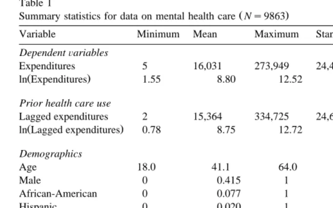
We illustrate the methods by analyzing Massachusetts Medicaid data, which were collected by the Massachusetts Division of Medical Assistance. The Medi-caid data set includes information on all Massachusetts MediMedi-caid claims from fiscal years 1991 and 1992. We limited the sample to the 9863 persons who were diagnosed with a severe mental illness and had at least one Medicaid claim in both years.

[image:14.595.46.388.67.280.2]

Table 1

Ž .

Summary statistics for data on mental health care Ns9863

Variable Minimum Mean Maximum Standard deviation Skewness

DependentÕariables

Expenditures 5 16,031 273,949 24,440 3.45

Ž .

ln Expenditures 1.55 8.80 12.52 1.42 y0.19

Prior health care use

Lagged expenditures 2 15,364 334,725 24,686 4.13

Ž .

ln Lagged expenditures 0.78 8.75 12.72 1.41 y0.14

Demographics

Age 18.0 41.1 64.0 11.7

Male 0 0.415 1 0.493

African-American 0 0.077 1 0.267

Hispanic 0 0.020 1 0.139

White 0 0.903 1 0.295

Health status

Schizophrenia 0 0.537 1 0.499

Major affective disorder 0 0.412 1 0.492

Other psychoses 0 0.050 1 0.218

Substance abuse 0 0.100 1 0.301

Ž .

US$16,000, but ranged from essentially zero to US$274,000 see Table 1 . One of the explanatory variables of interest was lagged expenditures, which had a similar distribution. Taking the logarithm of the dependent variable removed much of the skewness, although the skewness is negative and significantly different than zero. We also controlled for the standard demographic characteristics and health status. The patient population was 41.5% male, 89.5% white, 7.7% black, and 2% other race. The mean age was 41 years, and ranged from 18 to 64. All of the patients in the sample had one of the following diagnoses during the year:

Ž . Ž .

schizophrenia 53.7% , major affective disorder 41.3% , or other psychoses

Ž_{5.0% . Schizophrenia is considered the most serious of these conditions, followed}.

by major affective disorder and other psychoses. Substance abuse is a comorbidity strongly associated with mental health problems. Ten percent of our sample have a substance use comorbidity.

3.2. Results

good approximation to the finite sample distribution of the three estimands, and therefore do not report bootstrapping results. If the sample were relatively small, then the assumption of the normal distribution would be questionable, and bootstrapping would be preferred.

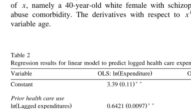
The results show, not surprisingly for this population with chronic disease, that logged annual health care expenditures are higher when lagged expenditures are

Ž .

higher see Table 2 . Expenditures are also higher for persons who are younger, female, white, schizophrenic, and have substance abuse comorbidity, results that are consistent with the literature. The heteroscedasticity regression, which predicts the squared residuals, has a low adjusted R2_{, but the estimated parameters of most}

of the explanatory variables are statistically significant. The LM form of the White

Ž1980 heteroscedasticity test, which regresses the squared estimated error term on.

the independent variables and their squares and interaction terms, is 106.5, leading

Ž

to rejection of the null hypothesis of homoscedasticity see second column of

.

[image:15.595.47.383.323.515.2]

Table 2 . For this example, we do not include squared terms or interaction terms, but it would be straightforward to do so. The results are shown for specific values of x, namely a 40-year-old white female with schizophrenia and no substance abuse comorbidity. The derivatives with respect to xk are for the continuous variable age.

Table 2

Regression results for linear model to predict logged health care expenditures 2

Ž .

Variable OLS: ln Expenditure OLS:´ˆ

) ) ) )

Ž . Ž .

Constant 3.39 0.11 2.23 0.26

Prior health care use

) ) ) )

Ž . Ž . Ž .

ln Lagged expenditures 0.6421 0.0097 y0.077 0.026

Demographics

) ) ) )

Ž . Ž .

Age y0.00374 0.00096 y0.0123 0.0020

) ) ) )

Ž . Ž .

Male y0.105 0.023 0.129 0.049

) )

Ž . Ž .

African-American y0.055 0.045 0.333 0.095

) ) )

Ž . Ž .

Hispanic y0.133 0.064 y0.315 0.098

Health status

) )

Ž . Ž .

Major affective disorder y0.126 0.022 y0.056 0.047 )

Ž . Ž .

Other psychoses y0.132 0.056 0.25 0.13

) )

Ž . Ž .

Substance abuse 0.542 0.035 y0.108 0.068

N 9863 9863

2

Adjusted R 0.45 0.01

The reference category is a white female with schizophrenia and no substance abuse comorbidity. Robust standard errors are corrected for heteroscedasticity using Huber–White robust standard errors.

)

Statistically significant at the 5% level. ) )

[image:16.595.48.384.78.182.2]

Table 3

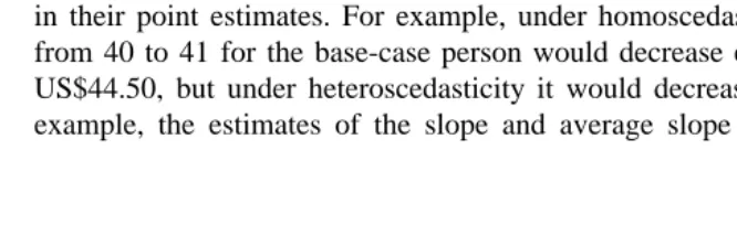
Computation of the conditional mean of y, the slope of y, the average slope of y, and their standard errors for the normal linear model

Assume hetero- Estimate Standard error scedasticity

Ž . w x

f x sE yNx No 11,884 264

Yes 11,667 314

k k

Ž . w x

Ef xrEx sEE yNxrEx No y44.5 11.7

Yes y115.4 17.1

k k

w Ž . x w w x x

EEf xrEx sEEE yNxrEx No y66.6 24.6

Yes y170.6 24.5

Calculations are for a 40-year-old white female with schizophrenia and no substance abuse comorbid-ity. Derivatives are with respect to age.

The three estimands are calculated both with and without the assumption of heteroscedasticity to show the importance of controlling for it in the normal linear

Ž .

model see Table 3 . The results show standard errors that are relatively small when compared to the magnitude of the three estimates. The estimated expendi-tures are slightly less than US$12,000, with a standard error of US$264 under homoscedasticity. The slope and the average slope in particular are quite different in their point estimates. For example, under homoscedasticity an increase in age from 40 to 41 for the base-case person would decrease expected expenditures by US$44.50, but under heteroscedasticity it would decrease by US$115.40. In our example, the estimates of the slope and average slope are biased towards zero

Table 4

Computation of the conditional mean of y, the slope of y, the average slope of y, and their standard errors for the nonparametric model

Assume hetero- Estimate Standard error scedasticity

Ž . w x

f x sE yNx No 12,296 327

Yes 12,044 300

k k

Ž . w x

Ef xrEx sEE yNxrEx No y46.0 12.0

Yes y131.1 16.9

k k

w Ž . x w w x x

EEf xrEx sEEE yNxrEx No y60.6 15.5

Yes y144.9 20.2

[image:16.595.50.383.431.533.2]

when heteroscedasticity is ignored, and the bias is large enough that the estimate without controlling for heteroscedasticity falls outside of the 95% confidence interval. This example shows the importance of controlling for heteroscedasticity both in the point estimate and in the standard error.

Ž

The three estimands are also calculated for the nonparametric model see Table

.

4 . The pattern of results is similar. Controlling for heteroscedasticity is clearly important for both the point estimates and the standard errors. The point estimates for the slope and average slope are much larger in absolute value after controlling for heteroscedasticity. The standard errors for all three stastistics are quite different after controlling for heteroscedasticity, and in two of the cases are larger.

In this example, however, the difference between the results for the normal and nonparametric models is small. Comparisons between Tables 3 and 4 show qualitatively similar results. In our example, the residuals are approximately normal, so the nonparametric model is not different from the normal model. In other data sets, however, the nonparametric model may be more appropriate and could give quite different results.

4. Conclusion

The use of the log-transformed dependent variable in applied economics creates

w x

a potential bias when computing estimates of E yNx on the original scale, if the

error term either does not have a normal distribution or is heteroscedastic. Estimates on the original scale should be reported with standard errors, like all estimated values. One reason that the calculation of standard errors is not common is that the equations are not commonly known. This paper provides equations for the general case of error terms that have any distribution and are heteroscedastic, as well as for simpler cases. Another reason is that computing the standard errors is not automatically done in software. The authors will provide sample programs in Stata to compute the standard errors upon request.

Acknowledgements

Appendix A

A.1. Formulas for the normal linear model

For the normal linear model the formulas for Step III are:

X _ˆ X

x bq0.5 xaˆ

Ž .

m

ˆ

x se scalar

ˆ

bk,a

ˆ

k scalars, estimated parameters for xk

ek vector of 0s, with 1 in the k th

position

Em

ˆ

Ž .

x

ˆ

Ž .Ž .

sm

ˆ

x bkq0.5a

ˆ

k scalar

k Ex

Em

ˆ

Ž .

x

Ž .

sm

ˆ

x x vector

Eb

Em

ˆ

Ž .

x

Ž .

s0.5m

ˆ

x x vector

Ea

2

Em

ˆ

Ž .

x Em

ˆ

Ž .

x

Ž .

s xqm

ˆ

x ek vector

k k

EbEx Ex

2

Em

ˆ

Ž .

x Em

ˆ

Ž .

x

s0.5 xqm

ˆ

Ž .

x ek vector

k

ž

k

/

EaEx Ex

2 2

Em

Ž .

x 1 _N Em

ˆ

Ž

xi

.

ˆ

E _EbE k s_NÝis1 k vector, simple average

x EbEx

2 2

Em

Ž .

x 1 _N Em

ˆ

Ž

xi

.

ˆ

E _EaExk s _NÝ_is1 _EaExk vector, simple average

A.2. Formulas for the normal nonlinear model

For the normal nonlinear model the formulas for Step III are:

ˆ

ŽhŽx,b.q0.5 sŽx,aˆ..

Ž .

m

ˆ

x se scalar

ˆ

Em

ˆ

Ž .

x Eh x,

Ž

b

.

Ž .

sm

ˆ

x vector

Eb Eb

Em

ˆ

Ž .

x Es x,

Ž

a

ˆ

.

Ž .

sm

ˆ

x 0.5 vector

Ea Ea

ˆ

Em

ˆ

Ž .

x Eh x,

Ž

b

.

Es x,

Ž

a

ˆ

.

Ž .

sm

ˆ

x q0.5 scalar

k k k

2

ˆ

2

ˆ

Em

ˆ

Ž .

x Em

ˆ

Ž .

x Eh x,

Ž

b

.

Es x,

Ž

a

ˆ

.

E h x,

Ž

b

.

Ž .

s q0.5 qm

ˆ

x

X

k _Eb k k k

Ex Eb Ex Ex Ex Eb

vector

2

ˆ

2

Em

ˆ

Ž .

x Em

ˆ

Ž .

x Eh x,

Ž

b

.

Es x,

Ž

a

ˆ

.

E s x,

Ž

a

ˆ

.

Ž .

s q0.5 q0.5m

ˆ

x

X

k _Ea k k k

Ex Ea Ex Ex Ex Ea

vector

A.3. Formulas for the nonparametric model with homoscedasticity

For the nonparametric model with homoscedasticity the formulas for Step III are:

2

ˆ

N

ˆ

Em

ˆ

Ž .

x _sm

ˆ

Ž .

_x Eh x ,

Ž

b

.

_yehŽx ,bˆ.1

Ý

ž

_e´ˆiEh x ,

Ž

i b

.

/

_vector

Eb Eb N_is1 Eb

The second term in the first derivative above arises from the fact that the

ˆ

residuals ´

ˆ

i are estimated and hence depend on the parameter estimate b.

2

ˆ

ˆ

Em

ˆ

Ž .

x E h x ,

Ž

b

.

Em

ˆ

Ž .

x Eh x ,

Ž

b

.

sm

ˆ

Ž .

x q vector

k k _Eb k

Ex Eb Ex Eb Ex

2 N 2

ˆ

Em

Ž .

x 1 E h x ,

Ž

i b

.

ˆ

E _k s

Ý

y_{i k} vector

N

Ex Eb _is1 Ex Eb

Four of the S’s are estimated by running a simple regression, saving the vector of regression coefficients, and dividing them by N. The part of the dependent variable that is not ´

ˆ

i orh

ˆ

i must have its mean subtracted before multiplying by the estimated error.

Estimated Dependent variable Independent

coefficients variable

ˆ

Ž Ž

ˆ

. . Ž

ˆ

.

S1 Db exp h x,b q´

ˆ

i =´

ˆ

i Eh x ,i b rEb

ˆ

Ž Ž

ˆ

. . Ž

ˆ

.

S2 Db exp h x,b q´

ˆ

i Eh x ,i b rEb

k

ˆ

Ž .

=Eh x,b rEx =´

ˆ

i y1

ˆ

w Ž Ž

ˆ

. . Ž

ˆ

.

S3 Db N Ýjexp h x ,j b q´

ˆ

i Eh x ,i b rEb

k

ˆ

Ž . x

=Eh x ,j b rEx =´

ˆ

i k

ˆ

w Ž

ˆ

. x Ž

ˆ

.

Four of the S’s are estimated by computing the sample variance divided by N

Žscalar ..

Estimated variance Sample variance of

ˆ

Ž Ž

ˆ

. .

S_1DD exp h x,b q´_i

k

ˆ

Ž Ž

ˆ

. .Ž Ž

ˆ

. .

S2 DD exp h x,b q´i Eh x,b rEx

y1 k

ˆ

Ž Ž

ˆ

. . Ž

ˆ

.

S3DD N Ýjexp h x ,j b q´

ˆ

i = Eh x ,j b rEx

k

ˆ

Ž Ž

ˆ

. .

S_m y_i Eh x ,_i b rEx

A.4. Formulas for the nonparametric model with heteroscedasticity

For the nonparametric model with heteroscedasticity the formulas for Step III are:

N

ˆ

Em

ˆ

Ž .

x 1 Egi

Ž

x ,b,a

ˆ

.

s

Ý

vector

Eb N_is1 Eb

N

ˆ

Em

ˆ

Ž .

x 1 Egi

Ž

x ,b,a

ˆ

.

s

Ý

vector

Ea N_is1 Ea

2 N 2

ˆ

Em

ˆ

Ž .

x 1 E gi

Ž

x ,b,a

ˆ

.

s

Ý

vector

k _N k

Ex Eb _is1 Ex Eb

2 N 2

ˆ

Em

ˆ

Ž .

x 1 E gi

Ž

x ,b,a

ˆ

.

s

Ý

vector

k k

N

Ex Ea _is1 Ex Ea

2 N

ˆ

Em

Ž .

x 1 Eqi

Ž

b,a

ˆ

.

ˆ

E _k s

Ý

ž

/

vector

N Eb

Ex Eb _is1

2 N

ˆ

Em

Ž .

x 1 Eqi

Ž

b,a

ˆ

.

ˆ

E _k s

Ý

ž

/

vector.

N Ea

Ex Ea _is1

y1

N _{Eh x ,}

Ž

_b

ˆ

.

_{Eh x ,}

Ž

_b

ˆ

.

N _{Eh x ,}

Ž

_b

ˆ

.

_{Es x ,}

Ž

_a

ˆ

.

i i i i

ˆ

Sb as

ž

Ý

X

/ ž

Ý

´ h

ˆ ˆ

i i X

/

Eb Eb Eb Ea

is1 is1

y1

N _{Es x ,}

Ž

_a

ˆ

.

_{Es x ,}

Ž

_a

ˆ

.

i i

=

ž

Ý

X

/

matrix

Ea Ea

is1

dependent variable that is not ´

ˆ

i or h

ˆ

i must have its mean subtracted before multiplying by the estimated error.

Estimated Dependent variable Independent

coefficient variable

ˆ

Ž

ˆ

. Ž

ˆ

.

S1Db g x,i b,a

ˆ

=´

ˆ

i Eh x ,i b rEb

ˆ

Ž

ˆ

. Ž .

S1Da g x,i b,a

ˆ

=h

ˆ

i Es x ,i a

ˆ

rEa

k

ˆ

Ž Ž

ˆ

. . Ž

ˆ

.

S2 Db Eg x,i b,a

ˆ

rEx =´

ˆ

i Eh x ,i b rEb

k

ˆ

Ž Ž

ˆ

. . Ž .

S2 Da Eg x,i b,a

ˆ

rEx =h

ˆ

i Es x ,i a

ˆ

rEa

y1 k

ˆ

Ž Ž

ˆ

. . Ž

ˆ

.

S3Db N ÝjEg x ,i jb,a

ˆ

rEx =´

ˆ

i Eh x ,i b rEb

y1 k

ˆ

Ž Ž

ˆ

. . Ž .

S3Da N ÝjEg x ,i jb,a

ˆ

rEx =h

ˆ

i Es x ,i a

ˆ

rEa

ˆ

Ž

ˆ

. Ž

ˆ

.

Sqb qi b,a

ˆ

=´

ˆ

i Eh x ,i b rEb

ˆ

Ž

ˆ

. Ž .

Sqa qi b,a

ˆ

=h

ˆ

i Es x ,i a

ˆ

rEa

Four of the S’s are estimated by computing the sample variance divided by N

Ž_{scalar .}.

Estimated variance Sample variance of

ˆ

Ž

ˆ

.

S1DD g x,i b,a

ˆ

k

ˆ

Ž

ˆ

.

S2 DD Eg x,i b,a

ˆ

rEx

y1 k

ˆ

Ž

ˆ

.

S3DD N ÝjEg x ,i jb,a

ˆ

rEx

ˆ

Ž

ˆ

.

Sm qi b,a

ˆ

A.5. Proof of asymptotic independence

ˆ

Let b denote the least squares estimator of the regression

ln y

Ž .

i sh x ,

Ž

i b

.

q´i is1,2, . . . , N. Then applying a Taylor expansion, we obtain

y1

N _{Eh x ,}

Ž

_b

.

_{Eh x ,}

Ž

_b

.

N _{Eh x ,}

Ž

_b

.

i i i _{y0 .5}

ˆ

bybs

ž

Ý

X

/

Ý

´iqop

Ž

N

.

.

Eb Eb Eb

is1 is1

Ž .

See Amemiya 1985 for a derivation. Let ´

ˆ

i denote the least squares residuals. Note that

2

We can write

´2_{ss x ,}

Ž

_a

.

_qh

i i i

wherehi is the error term. Let a

ˆ

denote the least squares estimator from

´2_s

s x ,

Ž

a

.

qh)

ˆ

i i i

Applying the first-order Taylor series approximation, we obtain

y1

N _{Es x ,}

Ž

_a

.

_{Es x ,}

Ž

_a

.

N _{Es x ,}

Ž

_a

.

i i i _{y0 .5}

a

ˆ

yas

ž

Ý

X

/

Ý

hiqop

Ž

N

.

.

Ea Ea Ea

is1 is1

ˆ

_{w x w} 3 _x

Note that the covariance between b and a

ˆ

depends on E ´ hi iNxi sE ´ hi iNx .i

3

ˆ

w x

For normal´i, E ´i Nxi s0, implying that b and a

ˆ

are asymptotically indepen-dent.

References

Amemiya, T., 1985. Advanced Econometrics. Harvard Univ. Press, Cambridge, MA.

Duan, N., 1983. Smearing estimate: a nonparametric retransformation method. J. Am. Stat. Assoc. 78, 605–610.

Duan, N. et al., 1983. A comparison of alternative models for the demand for medical care. J. Bus. Econ. Stat. 1, 115–126.

Duan, N. et al., 1984. Choosing between the sample selection model and the multi-part model. J. Bus. Econ. Stat. 2, 283–289.

Greene, W.H., 2000. Econometric Analysis. Prentice-Hall, Upper Saddle River, NJ.

Jones, A.M., Yen, S.T., 1999. A Box–Cox Double-Hurdle Model. Manchester School, in press. Manning, W.G., 1998. The logged dependent variable, heteroscedasticity, and the retransformation

problem. J. Health Econ. 17, 283–296.

Manning, W.G., Mullahy, J., 1999. Estimating Log Models: To Transform or not to Transform. University of Chicago working paper.

Mullahy, J., 1998. Much ado about two: reconsidering retransformation and the two-part model in health econometrics. J. Health Econ. 17, 247–282.