AEROTRIANGULATION SUPPORTED BY CAMERA STATION POSITION
DETERMINED VIA PHYSICAL INTEGRATION OF LIDAR AND SLR DIGITAL
CAMERA
E. Mitishita* M. Martins, J. Centeno, F. Hainosz
Department of Geomatics - Federal University of Parana, UFPR - Centro Politécnico - Setor de Ciências da Terra CEP 81531-990 -
Curitiba, Paraná, Brazil
Commission I, WG I/3
KEY WORDS: Photogrammetry; System Calibration; LIDAR; SLR Digital Camera, Aerotriangulation
ABSTRACT
Nowadays lidar and photogrammetric surveys have been used together in many mapping procedures due to their complementary characteristics. Lidar survey is capable to promptly acquire reliable elevation information that is sometimes difficult via photogrammetric procedure. On the other hand, photogrammetric survey is easily able to get semantic information of the objects. Accessibility, availability, the increasing sensor size and quick image acquisition and processing are properties that have raised the use of SLR digital cameras in photogrammetry. Orthoimage generation is a powerful photogrammetric mapping procedure, where the advantages of the integration of lidar and image datasets are very well characterized. However, to perform this application both datasets must be within a common reference frame. In this paper, a procedure to have digital images positioned and oriented in the same lidar frame via a combination of direct and indirect georeferencing is studied. The SLR digital camera was physically connected with the lidar system to calculate the camera station’s position in lidar frame. After that, the aerotriangulation supported by camera station’s position is performed to get image´s exterior orientation parameters (EOP).
1. INTRODUCTION
In the last decades, many photogrammetric mapping procedures were developed to promptly get reliable information from images. Together, airborne and orbital sensors were optimized to work with same objectives. Following these goals, lidar and digital camera integration are, nowadays, a powerful procedure to produce earth spatial information. Within this context, orthoimage production is a mapping procedure vastly applied by many photogrammetric companies in the world. However, to perform this procedure three basic datasets are necessary: a digital terrain model (DTM), which is conveniently extracted from lidar dataset via filter algorithms (for more details, consult Kraus and Pfeifer, 2001, Sithole and Vosseman, 2004), a set of interior orientation parameters (IOP) of the digital camera, determined via camera calibration procedure (more information can be found in Fraser, 1997, Habib et al., 2006 and Mitishita, et al., 2010) and a set of exterior orientation parameters (EOP) of the images within the same lidar frame.
Two main usual methods are applied to get EOPs within the lidar reference system. When the camera is not connected with the GNSS-Inertial system, an indirect georeferencing is performed to compute the image EOPs via aerotriangulation. In this scenario, which is the most studied, lidar data can be used as a source of photogrammetric control and different procedures were proposed to extract control for photogrammetric triangulation. Habib et al. (2004) and Habib et al. (2005) used
three-dimensional straight lines for the registration of photogrammetric and lidar data. A line is computed from the lidar dataset by intersecting two planar patches that are previously defined by least-square adjustment. Ghanma (2006), habib et al. (2007) and Shin et al. (2007) used lidar planar patches as a source of control for photogrammetric georeferencing. In these studies, a planar patch was defined by 3D raw lidar points that lie on the specific ground region (e. g., roof tops). Mitishita et al. (2008) used control points computed from the centroid of a rectangular roof that was easily found in images and in laser 3D point clouds. A set of lidar points that lie on the rectangular roof top are previously selected to perform the 3D lidar coordinates of the centroid. Mitishita et al. (2011) used distinct control points computed via lidar dataset. In this study the horizontal and vertical coordinates are extracted by interpolation procedure using the intensity image and lidar point cloud. The second procedure, when the digital camera is connected with the GNSS-Inertial systems, a Direct Georeferencing is applied. However, to perform this process, a system calibration is frequently required to refine the boresight misalignment and position offsets present in the system, due to the inexactnesses of the parameters used to connect distinct reference frame present in each sensor. More details about this methodology can be found in Brzezinska (1999), Cramer et al. (2000), Cramer (2003) and Yastikll and Jacobsen (2005).
methodologies explained before can be used to extract the EOP within lidar frame. The main condition is to have the digital camera physically connected to the lidar system, allowing the record of the instant the images are taken, within the IMU trajectory. After that, in a post processing using GNSS-IMU dataset, the coordinates of the camera station’s position (Xs, Ys, Zs) are calculated. Finally, using these coordinates as a constraint in a photogrammetric bundle adjustment, the image orientation parameters are computed.
In this paper, the coordinates of the camera station’s position, computed from the last methodology, are used as a control point to perform aerotriangulation procedures. Two groups of the experiments are evaluated. In the first, the IOP set from an “independent calibration” was considered to perform the aerotriangulation process. In the second, the aerotriangulation experiments are performed via a system calibration. The experiments are conducted to evaluate the obtained accuracies from the aerotriangulation processes with variation of four layouts of ground control points.
The following four sections contain information about the camera used in this research, procedures applied to connect the camera to lidar system and the camera calibrations results. Finally, in the last sections, the obtained results from the performed experiments are shown and discussed, as well as the conclusions and recommendations for future work.
2. USED CAMERA
The Kodak pro DCS-14n Single Lens Reflex (SLR) digital camera, mounted with 35 mm Nikon lens was used to carry out this research. The CMOS sensor has 14 million effective pixels. The type is 2/3” with the size: diagonal equal 43 mm; width equal 36 mm and height equal 24 mm. The pixel size is 0.0079 mm. The images used on this research have 4500 x 3000 pixels.
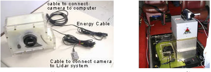
3. CAMERA AND LIDAR SYSTEM CONECTION Optech Airbone Laser Scanner ALTM 2050 was the lidar system used in this research. The camera was installed on the same lidar platform, allowing the use of the angular positions of the laser sensor as initial values to compute the images
orientation parameters. An acrylic box was specially built to fix the camera in the lidar platform. The Figure 1 shows these arrangements.
The camera is physically connected with the lidar system via RS232 serial cable to register, along the GNSS-IMU trajectory, the instants that the images are taken. Using post-processing techniques, the GNSS-IMU trajectory is calculated; inside this trajectory the positions and orientation of the sensor mirror are determined for the instants the images were taken. The lever arm was determined via topographic survey. The coordinates are shown in table 1. Using equations 1, the coordinates of the camera station can be computed. Due to the values of the roll and pitch rotation of the sensor mirror are close to zero, an approximated equations 2, 3 and 4 were used in this work. More details about the camera-and-lidar connection can be found in Martins, 2010.
ΔX (m) σ (m) ΔY (m) σ (m) ΔZ (m) σ (m) -0.039 0.007 0.180 0.007 -0.074 0.007 Table 1. Lever arm coordinates and their standard deviations.
����� ���=�
�� ��
���+�
(����,����ℎ,���) ×�∆�∆�
∆��
(1)
��=��+��� ��+ arctan�∆�∆���×�√∆�2+∆�2� (2)
��=��+��� ��+ arctan�∆�∆���×�√∆�2+∆�2� (3)
��=��+∆� (4)
�(����,����ℎ,���) = Attitude matrix from the orientation of the sensor mirror at the moment of the image was taken;
[������] = Coordinates of the camera station;
[������] = Coordinates of the sensor mirror at the moment of the image was taken;
[∆�∆�∆�] = Coordinates of the lever arm;
� = Azimuth of GNSS – IMU trajectory;
(a) (b)
4. CAMERA CALIBRATION
Two different types of IOP set are used to perform the experiments proposed in this research. The first set was computed via a bundle adjustment self-calibration using a 2D testfield. In this calibration, the camera was removed from the aircraft to take a set of convergent images of the 2D
testfield. The sixty target images were measured by manual monocular procedure. The self-calibration was performed using half of pixel (0.00395 mm) for the standard deviation of the image coordinates, and one millimeter for the standard deviation of the targets’ coordinates on the object space. The main results from the performed calibration, named as “independent calibration”, are shown in Table 2.
INDEPENDENT CALIBRATION (c)= Principal distance; (xp, yp)= Coordinates of principal point; (k1, K2)= Radial lens distortion; (σ)= Standard deviation. Table 2. The interior orientation parameters (IOP) computed in the “independent calibration that were significant on the
variance-covariance matrix.
The second type of IOP set is computed via “system calibration”. The aerotriangulation experiments used an aerial image block with twenty-three images acquired in two strips (almost coincident with opposite flight directions - approximately West-East and East-West). The flight height was close to 1,000 meters, resulting in a ground sample distance (GSD) close to 23 centimeters. The image block has forty-seven signalized control points and one hundred and fifty-three natural photogrammetric tie points. All signalized control points have 3D coordinates determined via precise GPS survey. Four layouts of control and check points are used to perform the system calibration experiments. In addition, the 3D coordinates of the camera station’s positions, computed via camera and lidar system integration, were used
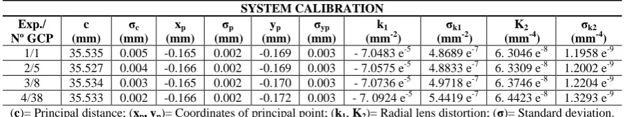
to minimize the correlation between a group of interior and exterior orientation parameters. The bundle adjustment self-calibrations were performed, using half of pixel (0.00395 mm) for the standard deviation of the image coordinates and one centimeter for the standard deviation of the ground coordinates of the control points and camera station’s positions. The value of one centimeter was the estimated precision of the GPS 3D coordinates of the control points and camera station’s positions. This procedure was considered, in this work, as “system calibration” to estimate the IOP set within the same work circumstances. The four IOP sets and theirs precisions that were computed in the system calibration experiments are shown in Table 3. More details about these calibrations can be found in Mitishita et al., 2010.
SYSTEM CALIBRATION (c)= Principal distance; (xp, yp)= Coordinates of principal point; (k1, K2)= Radial lens distortion; (σ)= Standard deviation. Table 3. The interior orientation parameters (IOP) computed in the “system calibration” that were significant on the
variance-covariance matrix.
5. AEROTRIANGULATION
The aerotriangulation experiments performed in this research can be separated in two groups. In the first, before the bundle adjustment procedure, the IOP set from an “independent calibration” was used to correct the measurements from the principal point displacement and the radial lens distortion. In the second, the IOP set is computed via bundle adjustment with self-calibration (system calibration). In both groups of the experiments, four configurations layout of ground control points were used. The first layout has only one ground control point located in the center of images block. The second has five control points, one in the center with four
one centimeter was the value adopted for the standard deviation of the 3D coordinates of the camera station and 3D ground coordinates of the control points. Half of one pixel (0.00395 mm) was the value adopted for the standard deviation of the image coordinates. The obtained precisions
from the residuals analysis performed in the eight experiments are shown in Table 4, and the main results from the accuracies study performed using check points are shown in Table 5.
RESIDUALS ANALYSIS Exp./
Nº GCP
Residuals in image coordinates (pixel)
Residuals in control points coordinates (mm)
Residuals in camera station’s coordinates (mm) Obtained results from aerotriangulation using IOP computed in “independent calibration”
Rmse x Rmse y Rmse X Rmse Y Rmse Z Rmse Xs Rmse Ys Rmse Zs (σo)
1/1 0.441 0.390 0.700 0.200 0.800 1.205 1.160 2.594 1.1566
2/5 0.459 0.406 1.490 1.262 1.281 1.420 1.230 1.735 1.2380
3/8 0.502 0.418 4.012 2.062 2.380 1.395 1.358 1.915 1.3911
4/38 0.625 0.471 4.270 2.382 2.208 1.842 1.465 3.901 1.8504
Obtained results from “system calibration”
Rmse x Rmse y Rmse X Rmse Y Rmse Z Rmse Xs Rmse Ys Rmse Zs (σo)
1/1 0.255 0.271 0.800 0.200 0.100 0.187 0.167 0.737 0.4605
2/5 0.261 0.274 1.064 1.210 0.648 0.199 0.169 0.800 0.4701
3/8 0.273 0.278 2.392 1.487 0.641 0.205 0.167 0.817 0.4933
4/38 0.331 0.314 2.928 2.163 0.608 0.171 0.230 1.031 0.6242
(σo)= A posteriori variance
Table 4. Main results of the residuals analysis performed in the experiments with aerotriangulation and system calibration
DISCREPANCIES ANALYSIS Experiments/
Nº Check points
Mean Values of the Discrepancies (m)
Root Mean Square Error of the Discrepancies (m) Obtained results from aerotriangulation using IOP computed in “independent calibration”
µ (DX) µ (DY) µ (DZ) Rmse (DX) Rmse (DY) Rmse (DZ)
1/46 -0.075 0.146 -0.760 0.395 0.997 0.890
2/42 -0.066 0.036 -0.884 0.192 0.161 0.997
3/39 -0.078 -0.048 -0.845 0.175 0.168 0.950
4/9 -0.005 -0.002 -0.579 0.107 0.096 0.718
Obtained results from “system calibration”
µ (DX) µ (DY) µ (DZ) Rmse (DX) Rmse (DY) Rmse (DZ)
1/46 0.028 -0.073 0.007 0.144 0.174 0.265
2/42 -0.002 0.047 -0.123 0.126 0.137 0.250
3/39 0.005 0.007 -0.060 0.122 0.119 0.213
4/9 0.002 0.008 -0.127 0.092 0.088 0.258
Table 5. Main results of the discrepancies analysis performed in the experiments with aerotriangulation and system calibration
Considering the results showed in Table 4, the values of the root mean square errors that were computed by the measurements residuals from the four bundle adjustment experiments via “system calibration” are smaller than those that were computed in the aerotriangulation experiments using IOP set from “independent calibration”. Despite the different variation, the measurement residuals were increased when the number of control points was enlarged. The aerotriangulation experiments performed with IOP from “independent calibration” produced biggest residuals. The better values of obtained precisions from the aerotriangulation with on the job calibration are expected because the procedure has the means to model the inaccuracies in the parameters involved. In contrast, if the measurements precisions, adopted in the bundle adjustment experiments (0.5 pixel for image measurement and 1 cm for X, Y, and Z coordinates of control points and camera
stations), are considered, the obtained precision from the experiments can be admitted as admissible. The residuals in image coordinates and residuals of 3D coordinates of control points and camera station’s positions have values of root mean square errors lower than the expected values in all performed experiments. On the other hand, when the check point study was performed, the obtained results from experiments (showed in Table 5) demonstrated that the obtained planimetric and vertical accuracies from two groups of experiments are different.
Considering the results showed in Table 5, the obtained accuracies from the aerotriangulation experiments with “system calibration” are better than the expected values of planimetric and vertical accuracies adopted in this work. The accuracies are very similar even though different configurations of control points are used. As can be seen in Table 3, very similar IOP sets are computed from different layout of control points, even though the layout with one control point positioned in the center of images block is used. In view of the obtained accuracies from the four aerotriangulation with “system calibration” experiments and the slight variability between their accuracies values, the experiment that used the layout of only one control point can be considered as the best procedure to perform the aerotriangulation of the image block tested in this research.
On the other hand, when the aerotriangulation supported by camera station’s position was performed without the “system calibration”, the obtained accuracies from the experiments performed did not have the same behavior as those that resulted from aerotriangulation with system calibration. In this scenario, the experiment using only one ground control point produced the worst planimetric accuracy. The root mean square errors from planimetric discrepancies are approximately four times greater than the expected planimetric accuracy (0.23 m). However, using other configuration layouts with more ground control points, the planimetric accuracy was improved. For example, the experiment, using layout with five ground control points, produced values of the root mean square errors of the planimetric discrepancies below 0.23 m but the planimetric accuracy is worse than that was produced in the experiments, using aerotriangulation with “system calibration”. On the other hand, the vertical accuracies from the performed experiments have different behavior. All of the performed experiments with four layouts of control points produced similar vertical accuracies. However, the obtained values are bigger than the value of the expected vertical accuracy, even though the layout with thirty-eight control point positioned in the images block is used. The obtained results from experiments in this scenario indicate that, for the bundle adjustment aerotriangulation without “system calibration” used in this research, the vertical accuracy is much more dependent of the accuracy of IOP set than the planimetric accuracy.
The experiments performed in this research demonstrated that the bundle adjustment aerotriangulation supported by the camera station coordinates requires a “system calibration” to increase planimetric and vertical accuracies in object point determination. Due to the high correlation, when a typical images block is used, with a group of interior and exterior parameters (Xo,Yo,Zo – camera station position versus (c, xo,yo) – focal length and principal point coordinates), the “system calibration” is able to refine some imprecision in system parameters, such as lever arms, photogrammetric refraction, focal length variation. However, the obtained results are highly correlated with the accuracies of GNSS/INS trajectory.
6. CONCLUSION AND RECOMMENDATION FOR FUTURE WORK
The aerotriangulation supported by camera station coordinates computed via physical integration of lidar and digital SLR camera has been studied and discussed. Two groups of the experiments were used to perform the bundle adjustment aerotriangulation with four different control point layouts. In the first, the IOP set from an “independent calibration” was considered to perform the aerotriangulation process. In the second, the aerotriangulation experiments are performed via a system calibration. The 3D coordinates of camera station position, computed from the camera and lidar systems integration, were used, as control points, in all experiments performed. One aerial image block with twenty-three images in two strips was captured by a Kodak DCS Pro 14n digital SLR. It was used to perform the proposed experiments. Considering the obtained results from the performed experiments, the following conclusions were drawn:
The aerotriangulation with the “system calibration” was a fundamental procedure to perform the bundle adjustment aerotriangulation supported by 3D coordinates of the camera station’s position. Accurate IOP values were the requirement to increase the horizontal and vertical precisions of the object point determination. Within this configuration, only one ground control point was enough to perform the bundle adjustment aerotriangulation with the “system calibration”. The planimetric and vertical accuracies were approximately equal in the experiments performed with four layouts of the ground control points.
The aerotriangulation experiments, using IOP set from the “independent calibration”, did not yield good results when only one ground control points was used. The planimetric and vertical accuracies that were obtained from this control point layout did not attain the tolerances adopted in this research. On the other hand, when the number of ground control points was increased, the planimetric accuracy increased too. In the experiment that used eight ground control points, the root mean square errors of the planimetric discrepancies are close to those computed in the same experiment that uses aerotriangulation with the “system calibration”. However, within this scenario, the vertical results did not change in the three experiments performed; the obtained results were worse and did not attain the vertical tolerance adopted in this research. These results attest that, for the methodology of bundle adjustment aerotriangulation used in this research, the vertical accuracy is much more dependent of the quality of IOP set than the planimetric accuracy.
adopted for the measurements in the bundle adjustment (0.5 pixel for images coordinates; 1 cm for coordinates of the control point and position of the camera station). Therefore, if only these parameters are considered for the mentioned experiments, the final results can be unacceptable because the horizontal and vertical accuracies do not validate them.
Future work will concentrate on a verification of the quality and performance of the IOP set from “system calibration”. It will be used to perform the bundle adjustment aerotriangulation supported by 3D coordinates of the camera station’s position, using image blocks captured in different scales, flight orientations and epoch. Additionally, the study to compute images orientation via the values of orientation of the sensor mirror will be conducted.
ACKNOWLEDGMENTS
We would like to thank the two Brazilian governmental agencies CNPq (The National Council for Scientific and Technologic Development) and CAPES (The Coordinating Agency for Advanced Training of High-Level Personnel) for their financial support of this research.
REFERENCES
CRAMER,M.,STALLMANN,D. AND HAALA,N., 2000. Direct georeferencing using GPS/Inertial exterior orientations for photogrammetric applications; International Archives of Photogrammetry and Remote Sensing, V. 33, part B3, pp. 198-205.
CRAMER M., 2003. GPS/inertial and digital aerial triangulation – recent test results. In. Photogrammetric Week 2003, Fritsch (ed.), Wichmann Verlag, Heidelberg, Germany, pp. 161-172.
FRASER, C.S., 1997. Digital camera self-calibration. ISPRS Journal of Photogrammetry and Remote Sensing, 52(4), pp. 149–159.
GHANMA, M., 2006. Integration of Photogrammetry and Lidar, PhD Thesis, University of Calgary, Department Of Geomatics Engineering, Calgary, Canada, 141 pages.
GREJNER-BRZEZINSKA, D. A., 1999. Direct Exterior Orientation of Airborne Imagery with GPS/INS System: Performance Analysis, Navigation, 46(4), pp. 261-270.
HABIB, A., GHANMA, M., and MITISHITA, E., 2004. Co-registration of photogrammetric and lidar data: methodology and case study, Brazilian Journal of Cartography, V-56/1, July 2004, pp. 1-13.
HABIB, A., GHANMA, M., MORGAN,M., AND AL-RUZOUQ,R., 2005. Photogrammetric and LiDAR data registration using
linear features, Photogrammetric Engineering and Remote Sensing, Vol. 71, No. 6, pp. 699-707.
HABIB, A., PULLIVELLI, A., MITISHITA, E., GHANMA, M. and EUI-MYOUNG KIM, 2006. Stability analysis of low-cost digital cameras for aerial mapping using different Georeferencing Techniques. Photogrammetric Record Journal, 21(113), pp. 29-43.
HABIB, A. F., BANG, K.I., SHIN, S.W., AND MITISHITA, E., 2007. LiDAR system self-calibration using planar patches from photogrammetric data, The 5th International Symposium on Mobile Mapping Technology, [CD-ROM], pp. 28-31 May, Padua, Italy.
KRAUS,K. AND PFEIFER,N.,2001. Advanced DTM generation from LiDAR data. International Archives of Photogrammetry, Remote Sensing and Spatial Information Sciences 34(3/W4), Annapolis, MD, USA, pp. 23-30.
MARTINS, M., 2010. Geração de ortoimagem a partir de georreferenciamento direto de imagens digitais aéreas de pequeno formato com dados lidar. 2010. 131 páginas, Dissertação (Mestrado em Ciências Geodésicas) – Setor de Ciências da Terra - Universidade Federal do Paraná – Curitiba – Paraná.
MITISHITA,E.,HABIB,A.,CENTENO,J.,MACHADO,A.,LAY, J., and WONG, C., 2008. Photogrammetric and Lidar data integration using the centroid of a rectangular building roof as a control point. The Photogrammetric Record, 23(121), pp 19-35.
MITISHITA, E., CORTES, J., CENTENO, J.,MACHADO, A, M., 2010. Study of stability analysis of the interior orientation parameters from the small-format digital camera using on-the-job calibration, In:
Vol. XXXVIII - part 1, Calgary, Canada, pp. 15-18, June (proceedings on CD-ROM).
MITISHITA, E., CORTES, J., CENTENO, J., 2011. Indirect georeferencing of digital SLR imagery using signalised lidar control points. The Photogrammetric Record 26(133), pp. 58-72.
SHIN,S.;HABIB,A.;GHANMA,M.;KIM,C.;KIM,E.-M., 2007. Algorithms for Multi-sensor and Multiprimitive Photogrammetric Triangulation. ETRI Journal. 2007, 29, pp. 411–420.
SITHOLE, G. AND VOSSELMAN G., 2004. Experimental comparison of filter algorithms for bare-Earth extraction from airborne laser scanning point clouds. ISPRS Journal of Photogrammetry and Remote Sensing 59(1-2), pp. 85-101.
YASTIKLI N., JACOBSEN K., 2005 Influence of System