Assessment of HICO data for Coastal Studies
Rimjhim Bhatnagar Singh* and Prakash Chauhan
Biological and Planetary Sciences and Applications Group, EPSA Space Applications Centre, ISRO, Ahmedabad
Corresponding Author, Email: [email protected]
ABSTRACT
Coastal waters, in particular, are the regions of high productivity and biodiversity. Detailed investigations of the variability within them can aid in understanding many biogeochemical processes. With the advent of hyperspectral remote sensing having large number of closely spaced channels and highly improved signal-to-noise ratio (SNR), the coastal applications are expected to increase and improve. In India, very less work is done in the field of coastal studies, let alone using hyperspectral remote sensing. HICO, onboard ISS, is the most recent addition to this family of instruments. So, a pilot study was conducted to assess HICO data for coastal studies especially in deriving the shallow water bathymetry estimates. The methodology for deriving bathymetry estimates is based on the different responses of shallow-water reflectance on depth and substrate type because with decreasing water depth in case 2 waters, the spectral contributions arriving from pure water reduce while from other OCAs increase. This variability is typically higher in the wavelength range 480 to 610nm. Using this wavelength range, bathymetric estimates were made at pixel level. Bathymetry estimates were found to vary from 1m to >12m. Spectral variability is clearly observed in the continuum removed spectral plots from waters of different depths and is reported in this paper.
KEYWORDS
Hyperspectral, HICO, Bathymetry, Spectra, Optically Complex Water,
INTRODUCTION
Coastal waters, in particular, are the regions of high productivity and biodiversity. Detailed investigations of the variability within them can aid in understanding many biogeochemical processes such as primary productivity (Cullen et al., 1997), carbon cycle etc and thus in coastal zone management (Nayak et al, 1996). They carry various optically active materials like phytoplankton, NAP, and CDOM. The incident light over water is absorbed and scattered by these materials. Hence, their varied concentration leads to the variability of natural as well as coastal waters and their apparent optical properties (AOPs).
In Case I waters, the optical properties are controlled by phytoplanktons and their associated degradations while in Case II waters which includes inland and coastal waters, their spectral characteristics are influenced by phytoplankton and other OCAs (Morel and Loisel, 1998) including varying proportions of sediments. With decreasing water depth, the spectral contributions arriving from pure water reduce while from other OCAs increase. Using this spectral information, gradients relating to biogeochemical concentrations of various types within water spread may be derived. In the past, many studies related to coastal applications have been done using broad band data. But, the hyperspectral data use for coastal studies is still in the nascent stage in India. With this purview in mind, space-borne hyperspectral data, HICO was investigated for coastal applications.
One of the primary requirements in the field of coastal studies is the bathymetry. Bathymetric or hydrographic charts usually
STUDY AREA
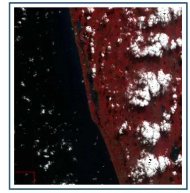
The study was conducted over a coastal part of the Arabian Sea region. The data analyzed was of 16th December 2013. Cloud patches were observed at many places within the scene, however, coastal regions, typically where this study was conducted, were largely cloud free. Figure 1 shows the FCC of the study area.
Figure 1: FCC of the study area (Bands selected are band 97, 60 and 42 corresponding to central wavelength
547.28nm, 650.38nm and 862.32nm respectively)
MATERIALS AND METHODS
In order to carry out this study, hyperspectral data was obtained from Hyperspectral Imager for Coastal Ocean (HICO). HICO sits over the International Space Station (ISS) and is largely meant for scientific research related to the coastal studies, though it may be very well used for terrestrial applications. Table 1 briefly describes the HICO specifications.
Table 1: HICO specifications
SNR >200:1 for 5% albedo target Nadir crosstrack
Saturation Does not saturate when viewing 95% albedo cloud
HICO data used in this study was dated 16th December 2013.
As shown in the FCC in figure 1, the image has many patches of clouds. Moreover, many non-water areas are also present. Both of these classes have to be removed before further analysis. So, three methods were investigated. First method was
based on slicing the image based on the radiance, second was based on Normalized Difference Water Index (NDWI) and the third on Modified Normalized Difference Water Index (MNDWI). The most appropriate technique was used to remove the cloudy pixels and the non-water pixels.
Masking of non-water area threshold. Also, NDWI and MNDWI were evaluated (Eq 1 and 1b). MNDWI (Xu, 2006) was particularly developed for removing the noise due to built-up land apart from background soil and vegetation effects.
NDWI= (Green-NIR)/(Green +NIR) (1a)
MNDWI= (Green-MIR)/(Green +MIR) (1b)
Once non-water areas from the image were masked, atmospheric correction was performed over the image using FLAASH module of ENVI image processing software. The reflectance image thus produced was used for bathymetry retrieval.
Bathymetry retrieval
Lyzenga (1978), in an extension to the Beer’s law of light attenuation with increasing water depth, showed that the observed reflectance could be expressed by depth and bottom albedo as follows:
RW= (Ad−R∞) exp (−gz) + R∞ (2)
Where R∞ is the water column reflectance if the water were
optically deep, Adis the bottom albedo, z is the depth, and g is a
(4)
In equations 3 and 4, N is total number of bands between 480 and 610 nm. Ri, jis the spectral reflectance of band j at pixel i , R0, jis the reference spectral reflectance of band j. A constant in
the formulae is added to ensure that the values are always positive.
From the above, water depth may be retrieved as:
(5)
Where k1 is a tuneable constant to scale the ratio to depth, n is a fixed constant that ensures the natural logarithms remain positive for every condition, and k0 is the offset.
After the bathymetry estimates, the image was density sliced as per the variations in water depth. The spectra for each class was then retrieved and analyzed.
RESULTS AND DISCUSSIONS
HICO data was provided in the ISS format which is not compatible with the generally used image processing software like ENVI IDL. Hence, the data was converted to geotiff format using SeaDas software. The data was provided in the digital counts, so radiance image was generated using the provided scaling factors. The radiance image and corresponding spectral plots for major land-cover types is shown in Figure 2 below.
.
Figure 2: Radiance image of the study area with corresponding spectral plots. Note that unit of radiance is
W/sq m/micrometer/steradian
Radiance plots for all the classes come in consensus with the observations from other sensors. A large amount of scattering in blue region is observed leading to an overall increase in radiance in the initial bands. Note that in both case 1 and case 2 waters not much spectral variability is observed in the radiance domain, although both the classes have immense difference in their constitution otherwise. The reflectance domain is expected to show the marked variability between the two classes. However, the prerequisite is masking of non-water regions before attempting reflectance retrieval. Hence, the
radiance image was density sliced and NDWI and MNDWI maps were generated (figure 3).
Figure 3: Density sliced radiance, NDWI and MNDWI images respectively
Broadly speaking, all the three methods of cloud making are able to mask out clouds an terrestrial areas. But, radiance based masking is highly subjective to the band slected for density slicing. So, this technique was dropped from comparison. When NDWI and MNDWI are carefully analyzed, it is observed that MNDWI outperforms the other two techniques of cloud masking as shown in figure 4.
Figure 4: Cross Comparison of NDWI and MNDWI in segregating non-water regions
Note that in figure 4, FCC of first set of images show water body, which is shown as clouds in NDWI image while MNDWI suitably classifies it as non-clouds. Also, in second set of images, NDWI is not able to identify thin cloud patches but MNDWI classifies them suitably. Consequently, MNDWI based non-water masking was selected in this study. Xu (2006) aslo showed better performance of MNDWI over NDWI in cases where background noise is large.
was performed using FLAASH module of ENVI image processing software. Figure 5a shows the atmospherically corrected image of the study area while figure 5b shows the MNDWI masked reflectance image of the study area.
Figure 5: (a) Atmospherically corrected image of the study area (b) MNDWI based masked reflectance image displaying ‘only water’ regions
Corresponding to figure 5, reflectance spectra were retrieved for case 1 as well as case 2 waters (shown in figure 6).
Figure 6: Reflectance plots for water
The reflectance goes to a high value of 0.4 or 40% in blue region, drops down to less than 5% and further low in higher wavelengths side.
In the two kinds of water, remarkable difference in magnitude as well as the pattern of the spectra is expected to be more pronounced in the wavelength region between 480 and 610nm. As a result, spectral plots within the same range are shown in figure 7 below. It may be noted that continuum removal was carried out to observe the distinct spectral variability between the two types of water.
Figure 7: Continuum removed reflectance plots for case 1 and case 2 waters within the wavelength range of 480 and
610nm
As was expected, the reflectance for case 2 waters is higher than case 1 waters primarily due to the dissolved optically active substances in them. Note that case 2 waters show high reflectance in ~550nm region as is shown by green vegetation. This indicates the presence of phytoplanktons.
Bathymetry Retrieval
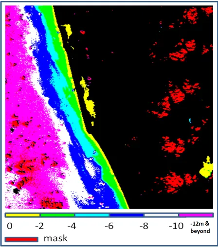
Bathymetry retrieval requires computations for the parameters CC and SC as per equations 3 and 4. Upon computing the two parameters and integrating them as in equation 5, bathymetry is retrieved (figure 8). Bathymetry map was density sliced into six classes showing water depth of ~-2m (shown in yellow colour) to <-10m (shown in magenta colour).
Figure 8: Density sliced bathymetry image
transect was chosen and corresponding bathymetric plot was obtained (Figure 9). Inland waters and coastal areas appear to be shallow (~1-3m) than a sharp gradient in depth is observed followed by almost uniform depth.
Figure 9: Bathymetry profile across the scene shown in inset
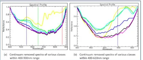
For each class of water the spectral plots were obtained and are shown in figure 10 below. It is evident that waters having variable depths show differences in their spectra also. Concurrent sample observations for chlorophyll content and suspended matter may be used to derive quantitative information from these spectra.
Figure 10: Continuum removed reflectance spectra of the various classes of density sliced bathymetric image
CONCLUSION
In this study, hyperspectral data from HICO instrument is assessed for coastal studies. In this direction, the data was first processed for removing the terrestrial and clouds components by using three techniques. MNDWI was found to be the best when compared with the other two techniques. The radiance plots for different target types were extracted and were found to fall in consensus with the standard observations. The data was then used for retrieving shallow water bathymetry. Bathymetry estimates were found to vary from ~1m to ~12m in depth. The spectra of case 1 and case 2 waters obtained from the density sliced bathymetry image showed large variability in reflectance domain especially in the 480-610nm range. However, the reflectance values match well with the standard observations. This implies that both in radiance and reflectance domain, the spectral characteristics of water in term of pattern and
amplitude show that HICO data can be very well used for quantitative coastal applications. The data can also be used for deriving shallow water bathymetry estimates useful for many navigation and climatic applications.
References
Conger, C. L. , E. J. Hochberg, C. H. Fletcher, and M. J. Atkinson. “Decorrelating remote sensing color bands from bathymetry in optically shallow waters,” IEEE Trans. Geosci.
Remote Sens., vol. 44, no. 6, pp. 1655–1660, Jun. 2006.
Cullen et al., 1997
http://www.ngdc.noaa.gov/mgg/global/ relief/ETOPO2/ETOPO2-2001
Loomis, M. J. “Depth derivation from the worldview-2 satellite using hyperspectral imagery,” M.S. thesis, Dept. Meteorol., Naval Postgraduate School, Monterey, CA, USA, 2009.
Lyzenga, D. R. “Passive remotesensing techniques for mapping water depth and bottom features,” Appl. Opt., vol. 17, no. 3, pp. 379–383, 1978.
Ma, Sheng, Zui Tao, Xiaofeng Yang, Yang Yu, Xuan Zhou, and Ziwei Li. “Bathymetry Retrieval from Hyperspectral Remote Sensing Data in Optical-Shallow Water”, IEEE Transactions On Geoscience And Remote Sensing, Vol. 52, No. 2, February 2014.
Morel and Loisel, 1998
National Geophysical Data Center Data announcement
88-MGG-02, Digital relief of the Surface of the Earth, Natl.
Oceanic and Atmos. Admin., US Dept. Commerce, Boulder, Colorado, USA, 1988.
National Geophysical Data Center 2-minute Gridded Global Relief Data (ETOPO2v2), Natl. Oceanic and Atmos. Admin.,
U. S. Dept. of Commerce,
(http://www.ngdc.noaa.gov/mgg/fliers/06mgg01.html), 2006.
Nayak Shailesh, P Chauhan, H.B. Chauhan, Anjali Bahuguna and A. N arendra Nath.”IRS-1C applications for Coastal Zone Mangement”, Current Science, Vol 70, No. 7, April 1996.
Stumpf, R. P., K. Holderied, and M. Sinclair. “Determination of water depth with high-resolution satellite imagery over variable bottom types,” Limnol. Oceanogr., vol. 48, no. 1, pp. 547–556, Jan. 2003.