543
Chapter 10
Spectroscopic Methods
Chapter Overview
Section 10A
Overview of Spectroscopy
Section 10B Spectroscopy Based on Absorption
Section 10C
UV/Vis and IR Spectroscopy
Section 10D
Atomic Absorption Spectroscopy
Section 10E
Emission Spectroscopy
Section 10F
Photoluminescent Spectroscopy
Section 10G
Atomic Emission Spectroscopy
Section 10H
Spectroscopy Based on Scattering
Section 10I
Key Terms
Section 10J
Chapter Summary
Section 10K
Problems
Section 10L
Solutions to Practice Exercises
A
n early example of a colorimetric analysis is Nessler’s method for ammonia, which was introduced in 1856. Nessler found that adding an alkaline solution of HgI2 and KI to a dilute solution of ammonia produces a yellow to reddish brown colloid, with the colloid’s color depending on the concentration of ammonia. By visually comparing the color of a sample to the colors of a series of standards, Nessler was able to determine the concentration of ammonia.10A Overview of Spectroscopy
he focus of this chapter is on the interaction of ultraviolet, visible, and infrared radiation with matter. Because these techniques use optical materi-als to disperse and focus the radiation, they often are identiied as optical spectroscopies. For convenience we will use the simpler term spectroscopy in place of optical spectroscopy; however, you should understand that we are considering only a limited part of a much broader area of analytical techniques.
Despite the diference in instrumentation, all spectroscopic techniques share several common features. Before we consider individual examples in greater detail, let’s take a moment to consider some of these similarities. As you work through the chapter, this overview will help you focus on
similarities between diferent spectroscopic methods of analysis. You will ind it easier to understand a new analytical method when you can see its relationship to other similar methods.
10A.1 What is Electromagnetic Radiation
Electromagnetic radiation—light—is a form of energy whose behavior is described by the properties of both waves and particles. Some properties of electromagnetic radiation, such as its refraction when it passes from one medium to another (Figure 10.1), are explained best by describing light as a wave. Other properties, such as absorption and emission, are better de-scribed by treating light as a particle. he exact nature of electromagnetic radiation remains unclear, as it has since the development of quantum mechanics in the irst quarter of the 20th century.1 Nevertheless, the dual
models of wave and particle behavior provide a useful description for elec-tromagnetic radiation.
WAVE PROPERTIESOF ELECTROMAGNETIC RADIATION
Electromagnetic radiation consists of oscillating electric and magnetic ields that propagate through space along a linear path and with a constant ve-locity. In a vacuum electromagnetic radiation travels at the speed of light, c, which is 2.997 92 � 108 m/s. When electromagnetic radiation moves through a medium other than a vacuum its velocity, v, is less than the speed of light in a vacuum. he diference between v and c is suiciently small (<0.1%) that the speed of light to three signiicant igures, 3.00 � 108 m/s, is accurate enough for most purposes.
he oscillations in the electric and magnetic ields are perpendicular to each other, and to the direction of the wave’s propagation. Figure 10.2
shows an example of plane-polarized electromagnetic radiation, consisting of a single oscillating electric ield and a single oscillating magnetic ield.
An electromagnetic wave is characterized by several fundamental prop-erties, including its velocity, amplitude, frequency, phase angle,
polariza-1 Home, D.; Gribbin, J. New Scientist 1991, 2 Nov. 30–33.
tion, and direction of propagation.2 For example, the amplitude of the
oscillating electric ield at any point along the propagating wave is
At =Aesin(2πνt+Φ)
where At is the magnitude of the electric ield at time t, Ae is the electric ield’s maximum amplitude, n is the wave’s frequency—the number of oscillations in the electric ield per unit time—and F is a phase angle, which accounts for the fact that At need not have a value of zero at t = 0. he identical equation for the magnetic ield is
At = Amsin(2πνt+Φ)
where Am is the magnetic ield’s maximum amplitude.
Other properties also are useful for characterizing the wave behavior of electromagnetic radiation. he wavelength, l, is deined as the distance between successive maxima (see Figure 10.2). For ultraviolet and visible electromagnetic radiation the wavelength is usually expressed in nanome-ters (1 nm = 10–9 m), and for infrared radiation it is given in microns (1
mm = 10–6 m). he relationship between wavelength and frequency is λ
ν = c
Another unit useful unit is the wavenumber, ν, which is the reciprocal of wavelength
ν λ = 1
Wavenumbers are frequently used to characterize infrared radiation, with the units given in cm–1.
2 Ball, D. W. Spectroscopy1994, 9(5), 24–25.
Figure 10.2 Plane-polarized electromagnetic radiation showing the oscillating electric ield in red and the oscil-lating magnetic ield in blue. he radiation’s amplitude, A, and its wavelength, l, are shown. Normally, elec-tromagnetic radiation is unpolarized, with oscillating electric and magnetic ields present in all possible planes perpendicular to the direction of propagation.
When electromagnetic radiation moves between diferent media—for example, when it moves from air into water—its frequency, n, remains constant. Because its velocity depends upon the medium in which it is traveling, the electromagnetic radiation’s wavelength, l, changes. If we replace the speed of light in a vacuum, c, with its speed in the medium, v, then the wavelength is
λ ν =v
his change in wavelength as light passes between two media explains the refrac-tion of electromagnetic radiarefrac-tion shown in Figure 10.1.
direction of propagation
elec
tr
ic field
mag netic field
λ
Example 10.1
In 1817, Josef Fraunhofer studied the spectrum of solar radiation, observ-ing a continuous spectrum with numerous dark lines. Fraunhofer labeled the most prominent of the dark lines with letters. In 1859, Gustav Kirch-hof showed that the D line in the sun’s spectrum was due to the absorption of solar radiation by sodium atoms. he wavelength of the sodium D line is 589 nm. What are the frequency and the wavenumber for this line?
S
OLUTIONhe frequency and wavenumber of the sodium D line are ν
λ
= = ×
× − = ×
− c 3 00 10
10 5 09 10
8
9
14 1
.
. m/s
589 m s
ν λ = =
× − × = ×
−
1 1
589 10
1
1 70 10
9
4 1
m
m
100 cm . cm
Practice Exercise 10.1
Another historically important series of spectral lines is the Balmer series of emission lines form hydrogen. One of the lines has a wavelength of 656.3 nm. What are the frequency and the wavenumber for this line? Click here to review your answer to this exercise.
PARTICLE PROPERTIESOF ELECTROMAGNETIC RADIATION
When matter absorbs electromagnetic radiation it undergoes a change in energy. he interaction between matter and electromagnetic radiation is easiest to understand if we assume that radiation consists of a beam of en-ergetic particles called photons. When a photon is absorbed by a sample it is “destroyed,” and its energy acquired by the sample.3 he energy of a
photon, in joules, is related to its frequency, wavelength, and wavenumber by the following equalities
E =hν=hc =hc
λ ν
where h is Planck’s constant, which has a value of 6.626 � 10–34 J .s.
Example 10.2
What is the energy of a photon from the sodium D line at 589 nm?
S
OLUTIONhe photon’s energy is
E =hc = × ⋅ × ×
−
λ
( .6 626 10 10
589 10
34 8
J s)(3.00 m/s)
− −
−
= ×
9
19
3 37 10
m . J
Figure 10.3 he electromagnetic spectrum showing the boundaries between diferent regions and the type of atomic or molecular transition responsible for the change in energy. he colored inset shows the visible spectrum. Source: modiied from Zedh (www.commons.wikipedia.org).
Practice Exercise 10.2
What is the energy of a photon for the Balmer line at a wavelength of 656.3 nm?
Click here to review your answer to this exercise.
THE ELECTROMAGNETIC SPECTRUM
he frequency and wavelength of electromagnetic radiation vary over many orders of magnitude. For convenience, we divide electromagnetic radiation into diferent regions—the electromagnetic spectrum—based on the type of atomic or molecular transition that gives rise to the absorption or emission of photons (Figure 10.3). he boundaries between the regions of the electromagnetic spectrum are not rigid, and overlap between spectral regions is possible.
10A.2 Photons as a Signal Source
In the previous section we deined several characteristic properties of elec-tromagnetic radiation, including its energy, velocity, amplitude, frequency, phase angle, polarization, and direction of propagation. A spectroscopic measurement is possible only if the photon’s interaction with the sample leads to a change in one or more of these characteristic properties.
Types of Atomic & Molecular Transitions
γ-rays: nuclear
X-rays: core-level electrons Ultraviolet (UV): valence electrons Visible (Vis): valence electrons Infrared (IR): molecular vibrations
Microwave: molecular roations; electron spin Radio waves: nuclear spin
γ-rays X-rays UV IR Microwave FM AM Long radio waves
Radio waves
Increasing Frequency (ν)
Increasing Wavelength (λ)
Visible Spectrum
Increasing Wavelength (λ) in nm
1024 1022 1020 1018 1016 1014 1012 1010 108 106 104 102 100
10-16 10-14 10-12 10-10 10-8 10-6 10-4 10-2 100 102 104 106 108
ν (s-1)
λ (nm)
400 500
We can divide spectroscopy into two broad classes of techniques. In one class of techniques there is a transfer of energy between the photon and the sample. Table 10.1 provides a list of several representative examples.
In absorption spectroscopy a photon is absorbed by an atom or mol-ecule, which undergoes a transition from a lower-energy state to a higher-energy, or excited state (Figure 10.4). he type of transition depends on the photon’s energy. he electromagnetic spectrum in Figure 10.3, for example, shows that absorbing a photon of visible light promotes one of the atom’s or molecule’s valence electrons to a higher-energy level. When an molecule absorbs infrared radiation, on the other hand, one of its chemical bonds experiences a change in vibrational energy.
Table 10.1 Examples of Spectroscopic Techniques Involving an Exchange of Energy
Between a Photon and the Sample
Type of Energy Transfer
Region of
Electromagnetic Spectrum Spectroscopic Techniquea
absorption g-ray Mossbauer spectroscopy
X-ray X-ray absorption spectroscopy
UV/Vis UV/Vis spectroscopy
atomic absorption spectroscopy
IR infrared spectroscopy
raman spectroscopy
Microwave microwave spectroscopy
Radio wave electron spin resonance spectroscopy nuclear magnetic resonance spectroscopy emission (thermal excitation) UV/Vis atomic emission spectroscopy
photoluminescence X-ray X-ray luorescence
UV/Vis fluorescence spectroscopy
phosphorescence spectroscopy atomic luorescence spectroscopy
chemiluminescence UV/Vis chemiluminescence spectroscopy
aTechniques discussed in this text are shown in
italics.
Figure 10.4 Simpliied energy diagram showing the absorption and emission of a photon by an atom or a molecule. When a photon of energy hn strikes the atom or molecule, absorption may occur if the difer-ence in energy, DE, between the ground state and the excited state is equal to the photon’s energy. An atom or molecule in an excited state may emit a photon and return to the ground state. he photon’s energy,
hn, equals the diference in energy, DE, between the
two states. ground state
exicted states
Ener
gy
hν ΔE = hν ΔE = hν hν
When it absorbs electromagnetic radiation the number of photons pass-ing through a sample decreases. he measurement of this decrease in pho-tons, which we call absorbance, is a useful analytical signal. Note that the each of the energy levels in Figure 10.4 has a well-deined value because they are quantized. Absorption occurs only when the photon’s energy, hn, matches the diference in energy, DE, between two energy levels. A plot of absorbance as a function of the photon’s energy is called an absorbance spectrum. Figure 10.5, for example, shows the absorbance spectrum of
cranberry juice.
When an atom or molecule in an excited state returns to a lower energy state, the excess energy often is released as a photon, a process we call emis-sion (Figure 10.4). here are several ways in which an atom or molecule may end up in an excited state, including thermal energy, absorption of a photon, or by a chemical reaction. Emission following the absorption of a photon is also called photoluminescence, and that following a chemi-cal reaction is chemi-called chemiluminescence. A typichemi-cal emission spectrum is shown in Figure 10.6.
Figure 10.5 Visible absorbance spectrum for cranberry juice. he anthocyanin dyes in cranberry juice absorb visible light with blue, green, and yellow wavelengths (see Figure 10.3). As a result, the juice appears red.
Molecules also can release energy in the form of heat. We will return to this point later in the chapter.
Figure 10.6 Photoluminescence spectrum of the dye coumarin 343, which is incorporated in a reverse micelle suspended in cy-clohexanol. he dye’s absorbance spectrum (not shown) has a broad peak around 400 nm. he sharp peak at 409 nm is from the laser source used to excite coumarin 343. he broad band centered at approximately 500 nm is the dye’s emission band. Because the dye absorbs blue light, a solution of coumarin 343 appears yellow in the absence of photoluminescence. Its photo-luminescent emission is blue-green. Source: data from Bridget Gourley, Department of Chemistry & Biochemistry, DePauw University).
400 450 500 550 600 650 700 750 0.0
0.2 0.4 0.6 0.8
wavelength (nm)
absor
banc
e
400 450 500 550 600 650
wavelength (nm)
emission in
tensit
y (ar
bitr
ar
In the second broad class of spectroscopic techniques, the electromag-netic radiation undergoes a change in amplitude, phase angle, polarization, or direction of propagation as a result of its refraction, relection, scatter-ing, difraction, or dispersion by the sample. Several representative spectro-scopic techniques are listed in Table 10.2.
10A.3 Basic Components of Spectroscopic Instruments
he spectroscopic techniques in Table 10.1 and Table 10.2 use instruments that share several common basic components, including a source of energy, a means for isolating a narrow range of wavelengths, a detector for measur-ing the signal, and a signal processor that displays the signal in a form con-venient for the analyst. In this section we introduce these basic components. Speciic instrument designs are considered in later sections.
SOURCESOF ENERGY
All forms of spectroscopy require a source of energy. In absorption and scattering spectroscopy this energy is supplied by photons. Emission and photoluminescence spectroscopy use thermal, radiant (photon), or chemi-cal energy to promote the analyte to a suitable excited state.
Sources of Electromagnetic Radiation. A source of electromagnetic
radia-tion must provide an output that is both intense and stable. Sources of electromagnetic radiation are classiied as either continuum or line sources. A continuum source emits radiation over a broad range of wavelengths, with a relatively smooth variation in intensity (Figure 10.7). A line source, on the other hand, emits radiation at selected wavelengths (Figure 10.8).
Table 10.3 provides a list of the most common sources of electromagnetic radiation.
Sources of hermal Energy. he most common sources of thermal energy
are lames and plasmas. Flames sources use the combustion of a fuel and an oxidant to achieve temperatures of 2000–3400 K. Plasmas, which are hot, ionized gases, provide temperatures of 6000–10 000 K.
Table 10.2 Examples of Spectroscopic Techniques That Do Not Involve an
Exchange of Energy Between a Photon and the Sample
Region of
Electromagnetic Spectrum Type of Interaction Spectroscopic Techniquea
X-ray difraction X-ray difraction
UV/Vis refraction refractometry
scattering nephelometry
turbidimetry
dispersion optical rotary dispersion a Techniques discussed in this text are shown in
italics.
You will ind a more detailed treatment of these components in the additional re-sources for this chapter.
Figure 10.7 Spectrum showing the emis-sion from a green LED, which provides continuous emission over a wavelength range of approximately 530–640 nm.
500 550 600 650
wavelength (nm)
Emission I
n
tensit
y (ar
bitr
ar
Chemical Sources of Energy Exothermic reactions also may serve as a source of energy. In chemiluminescence the analyte is raised to a higher-energy state by means of a chemical reaction, emitting characteristic radia-tion when it returns to a lower-energy state. When the chemical reacradia-tion results from a biological or enzymatic reaction, the emission of radiation is called bioluminescence. Commercially available “light sticks” and the lash of light from a irely are examples of chemiluminescence and biolu-minescence.
WAVELENGTH SELECTION
In Nessler’s original colorimetric method for ammonia, described at the beginning of the chapter, the sample and several standard solutions of am-monia are placed in separate tall, lat-bottomed tubes. As shown in Figure 10.9, after adding the reagents and allowing the color to develop, the analyst evaluates the color by passing natural, ambient light through the bottom of the tubes and looking down through the solutions. By matching the sample’s color to that of a standard, the analyst is able to determine the concentration of ammonia in the sample.
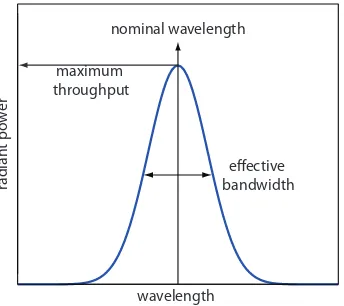
In Figure 10.9 every wavelength of light from the source passes through the sample. If there is only one absorbing species, this is not a problem. If two components in the sample absorbs diferent wavelengths of light, then a quantitative analysis using Nessler’s original method becomes impos-sible. Ideally we want to select a wavelength that only the analyte absorbs. Unfortunately, we can not isolate a single wavelength of radiation from a continuum source. As shown in Figure 10.10, a wavelength selector passes a narrow band of radiation characterized by a nominal wavelength, an effective bandwidth and a maximum throughput of radiation. he ef-fective bandwidth is deined as the width of the radiation at half of its maximum throughput.
Figure 10.8 Emission spectrum from a Cu hollow cathode lamp. his spectrum con-sists of seven distinct emission lines (the irst two difer by only 0.4 nm and are not resolved in this spectrum). Each emission line has a width of approximately 0.01 nm at ½ of its maximum intensity.
Table 10.3 Common Sources of Electromagnetic Radiation
Source Wavelength Region Useful for...
H2 and D2 lamp continuum source from 160–380 nm molecular absorption tungsten lamp continuum source from 320–2400 nm molecular absorption Xe arc lamp continuum source from 200–1000 nm molecular luorescence nernst glower continuum source from 0.4–20 mm molecular absorption globar continuum source from 1–40 mm molecular absorption nichrome wire continuum source from 0.75–20 mm molecular absorption hollow cathode lamp line source in UV/Visible atomic absorption Hg vapor lamp line source in UV/Visible molecular luorescence
laser line source in UV/Visible/IR atomic and molecular
absorp-tion, luorescence, and scattering
200 250 300 350 400
wavelength (nm)
Emission I
n
tensit
y (ar
bitr
ar
he ideal wavelength selector has a high throughput of radiation and a narrow efective bandwidth. A high throughput is desirable because more photons pass through the wavelength selector, giving a stronger signal with less background noise. A narrow efective bandwidth provides a higher res-olution, with spectral features separated by more than twice the efective bandwidth being resolved. As shown in Figure 10.11, these two features of a wavelength selector generally are in opposition. Conditions favoring a higher throughput of radiation usually provide less resolution. Decreasing the efective bandwidth improves resolution, but at the cost of a noisier signal.4 For a qualitative analysis, resolution is usually more important than
noise, and a smaller efective bandwidth is desirable. In a quantitative analy-sis less noise is usually desirable.
Wavelength Selection Using Filters. he simplest method for isolating a
narrow band of radiation is to use an absorption or interference filter. Absorption ilters work by selectively absorbing radiation from a narrow region of the electromagnetic spectrum. Interference ilters use construc-tive and destrucconstruc-tive interference to isolate a narrow range of wavelengths. A simple example of an absorption ilter is a piece of colored glass. A purple ilter, for example, removes the complementary color green from 500–560 nm. Commercially available absorption ilters provide efective bandwidths of 30–250 nm, although the throughput may be only 10% of the source’s emission intensity at the low end of this range. Interference ilters are more expensive than absorption ilters, but have narrower efective bandwidths, typically 10–20 nm, with maximum throughputs of at least 40%.
Wavelength Selection Using Monochromators. A ilter has one signiicant
limitation—because a ilter has a ixed nominal wavelength, if you need to make measurements at two diferent wavelengths, then you need to use two
4 Jiang, S.; Parker, G. A. Am. Lab.1981, October, 38–43.
Figure 10.9 Nessler’s original method for comparing the color of two solutions. Natural light passes upwards through the samples and stan-dards and the analyst views the solutions by looking down toward the light source. he top view, shown on the right, is what the analyst sees. To determine the analyte’s concentration, the analyst exchanges stan-dards until the two colors match.
Figure 10.10 Radiation exiting a wave-length selector showing the band’s nominal wavelength and its efective bandwidth.
side view
top view
wavelength
radian
t po
w
er
effective bandwidth nominal wavelength
diferent ilters. A monochromator is an alternative method for selecting a narrow band of radiation that also allows us to continuously adjust the band’s nominal wavelength.
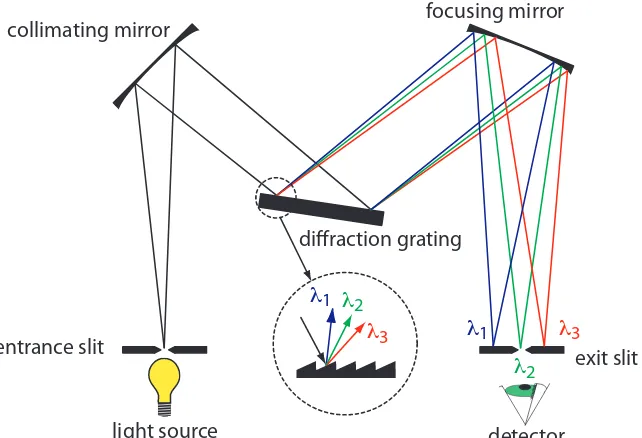
he construction of a typical monochromator is shown in Figure 10.12. Radiation from the source enters the monochromator through an entrance slit. he radiation is collected by a collimating mirror, which relects a par-allel beam of radiation to a difraction grating. he difraction grating is an optically relecting surface with a large number of parallel grooves (see insert to Figure 10.12). he difraction grating disperses the radiation and a second mirror focuses the radiation onto a planar surface containing an exit slit. In some monochromators a prism is used in place of the difrac-tion grating.
Radiation exits the monochromator and passes to the detector. As shown in Figure 10.12, a monochromator converts a polychromatic source of
Figure 10.11 Example showing the efect of the wavelength selector’s efective bandwidth on resolution and noise. he spectrum with the smaller efective bandwidth has a better resolution, allowing us to see the presence of three peaks, but at the expense of a noisier signal. he spectrum with the larger efective bandwidth has less noise, but at the expense of less resolution between the three peaks.
Figure 10.12 Schematic diagram of a monochromator that uses a difraction grating to disperse the radiation.
Polychromatic means many colored. Poly-chromatic radiation contains many difer-ent wavelengths of light.
wavelength
sig
nal
wavelength
sig
nal
larger effective bandwidth smaller effective bandwidth
λ1 λ3
λ2
λ1 λ2
λ3
entrance slit exit slit
collimating mirror
diffraction grating
focusing mirror
radiation at the entrance slit to a monochromatic source of inite efective bandwidth at the exit slit. he choice of which wavelength exits the mono-chromator is determined by rotating the difraction grating. A narrower exit slit provides a smaller efective bandwidth and better resolution, but allows a smaller throughput of radiation.
Monochromators are classiied as either ixed-wavelength or scanning. In a ixed-wavelength monochromator we select the wavelength by manu-ally rotating the grating. Normmanu-ally a ixed-wavelength monochromator is used for a quantitative analysis where measurements are made at one or two wavelengths. A scanning monochromator includes a drive mechanism that continuously rotates the grating, allowing successive wavelengths to exit from the monochromator. Scanning monochromators are used to acquire spectra, and, when operated in a ixed-wavelength mode, for a quantitative analysis.
Interferometers. An interferometer provides an alternative approach
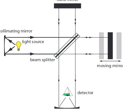
for wavelength selection. Instead of iltering or dispersing the electromag-netic radiation, an interferometer allows source radiation of all wavelengths to reach the detector simultaneously (Figure 10.13). Radiation from the source is focused on a beam splitter that relects half of the radiation to a ixed mirror and transmits the other half to a movable mirror. he radiation recombines at the beam splitter, where constructive and destructive inter-ference determines, for each wavelength, the intensity of light reaching the detector. As the moving mirror changes position, the wavelengths of light experiencing maximum constructive interference and maximum destruc-tive interference also changes. he signal at the detector shows intensity as a function of the moving mirror’s position, expressed in units of distance or time. he result is called an interferogram, or a time domain spectrum. Monochromatic means one color, or one
wavelength. Although the light exiting a monochromator is not strictly of a single wavelength, its narrow efective band-width allows us to think of it as mono-chromatic.
Figure 10.13 Schematic diagram of an inter-ferometers.
light source
detector fixed mirror
moving mirror beam splitter
collimating mirror
he time domain spectrum is converted mathematically, by a process called a Fourier transform, to a spectrum (also called a frequency domain spec-trum) showing intensity as a function of the radiation’s energy.
In comparison to a monochromator, an interferometer has two sig-niicant advantages. he irst advantage, which is termed Jacquinot’s ad-vantage, is the higher throughput of source radiation. Because an inter-ferometer does not use slits and has fewer optical components from which radiation can be scattered and lost, the throughput of radiation reaching the detector is 80–200� greater than that for a monochromator. he result is less noise. he second advantage, which is called fellgett’s advantage, is a savings in the time needed to obtain a spectrum. Because the detector monitors all frequencies simultaneously, an entire spectrum takes approxi-mately one second to record, as compared to 10–15 minutes with a scan-ning monochromator.
DETECTORS
In Nessler’s original method for determining ammonia (Figure 10.9) the analyst’s eye serves as the detector, matching the sample’s color to that of a standard. he human eye, of course, has a poor range—responding only to visible light—nor is it particularly sensitive or accurate. Modern detectors use a sensitive transducer to convert a signal consisting of photons into an easily measured electrical signal. Ideally the detector’s signal, S, is a linear function of the electromagnetic radiation’s power, P,
S=kP+D
where k is the detector’s sensitivity, and D is the detector’s dark current, or the background current when we prevent the source’s radiation from reaching the detector.
here are two broad classes of spectroscopic transducers: thermal trans-ducers and photon transtrans-ducers. Table 10.4 provides several representative examples of each class of transducers.
he mathematical details of the Fourier transform are beyond the level of this textbook. You can consult the chapter’s additional resources for additional infor-mation.
Transducer is a general term that refers to any device that converts a chemical or physical property into an easily measured electrical signal. he retina in your eye, for example, is a transducer that converts photons into an electrical nerve impulse.
Table 10.4 Examples of Transducers for Spectroscopy
Transducer Class Wavelength Range Output Signal
phototube photon 200–1000 nm current
photomultiplier photon 110–1000 nm current
Si photodiode photon 250–1100 nm current
photoconductor photon 750–6000 nm change in resistance
photovoltaic cell photon 400–5000 nm current or voltage
thermocouple thermal 0.8–40 mm voltage
thermistor thermal 0.8–40 mm change in resistance
pneumatic thermal 0.8–1000 mm membrane displacement
Photon Transducers. Phototubes and photomultipliers contain a photo-sensitive surface that absorbs radiation in the ultraviolet, visible, or near IR, producing an electrical current proportional to the number of photons reaching the transducer (Figure 10.14). Other photon detectors use a semi-conductor as the photosensitive surface. When the semisemi-conductor absorbs photons, valence electrons move to the semiconductor’s conduction band, producing a measurable current. One advantage of the Si photodiode is that it is easy to miniaturize. Groups of photodiodes may be gathered to-gether in a linear array containing from 64–4096 individual photodiodes. With a width of 25 mm per diode, for example, a linear array of 2048
pho-todiodes requires only 51.2 mm of linear space. By placing a photodiode array along the monochromator’s focal plane, it is possible to monitor
simultaneously an entire range of wavelengths.
hermal Transducers. Infrared photons do not have enough energy to
pro-duce a measurable current with a photon transpro-ducer. A thermal transpro-ducer, therefore, is used for infrared spectroscopy. he absorption of infrared pho-tons by a thermal transducer increases its temperature, changing one or more of its characteristic properties. A pneumatic transducer, for example, is a small tube of xenon gas with an IR transparent window at one end and a lexible membrane at the other end. Photons enter the tube and are absorbed by a blackened surface, increasing the temperature of the gas. As the temperature inside the tube luctuates, the gas expands and contracts and the lexible membrane moves in and out. Monitoring the membrane’s displacement produces an electrical signal.
Signal Processors
A transducer’s electrical signal is sent to a signal processor where it is displayed in a form that is more convenient for the analyst. Examples of signal processors include analog or digital meters, recorders, and comput-ers equipped with digital acquisition boards. A signal processor also is used to calibrate the detector’s response, to amplify the transducer’s signal, to remove noise by iltering, or to mathematically transform the signal.
10B Spectroscopy Based on Absorption
In absorption spectroscopy a beam of electromagnetic radiation passes through a sample. Much of the radiation passes through the sample without a loss in intensity. At selected wavelengths, however, the radiation’s intensity is attenuated. his process of attenuation is called absorption.
10B.1 Absorbance Spectra
here are two general requirements for an analyte’s absorption of electro-magnetic radiation. First, there must be a mechanism by which the radia-tion’s electric ield or magnetic ield interacts with the analyte. For ultra-Figure 10.14 Schematic of a
photomulti-plier. A photon strikes the photoemissive cathode producing electrons, which ac-celerate toward a positively charged dyn-ode. Collision of these electrons with the dynode generates additional electrons, which accelerate toward the next dynode. A total of 106–107 electrons per photon eventually reach the anode, generating an electrical current.
If the retina in your eye is a transducer, then your brain is a signal processor.
hν
photoemissive cathode dynode
anode
violet and visible radiation, absorption of a photon changes the energy of the analyte’s valence electrons. A bond’s vibrational energy is altered by the absorption of infrared radiation.
he second requirement is that the photon’s energy, hn, must exactly equal the diference in energy, DE, between two of the analyte’s quantized energy states. Figure 10.4 shows a simpliied view of a photon’s absorption, which is useful because it emphasizes that the photon’s energy must match the diference in energy between a lower-energy state and a higher-energy state. What is missing, however, is information about what types of energy states are involved, which transitions between energy states are likely to occur, and the appearance of the resulting spectrum.
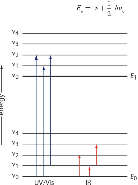
We can use the energy level diagram in Figure 10.15 to explain an absor-bance spectrum. he lines labeled E0 and E1 represent the analyte’s ground (lowest) electronic state and its irst electronic excited state. Superimposed on each electronic energy level is a series of lines representing vibrational energy levels.
INFRARED SPECTRAFOR MOLECULESAND POLYATOMIC IONS
he energy of infrared radiation produces a change in a molecule’s or a polyatomic ion’s vibrational energy, but is not suicient to efect a change in its electronic energy. As shown in Figure 10.15, vibrational energy levels are quantized; that is, a molecule may have only certain, discrete vibrational energies. he energy for an allowed vibrational mode, En, is
Eν= +v 1 hν
2 0
Figure 10.3 provides a list of the types of atomic and molecular transitions associ-ated with diferent types of electromag-netic radiation.
Figure 10.15 Diagram showing two electronic energy levels (E0 and E1), each with ive vibrational energy levels (n0–n4). Absorption of ultraviolet and visible radiation leads to a change in the analyte’s electronic energy levels and, possibly, a change in vibrational energy as well. A change in vibrational energy without a change in electronic energy levels occurs with the absorption of infrared radiation.
E0
E1
ν0
ν1
ν2
ν3
ν4
ν0
ν1
ν2
ν3
ν4
UV/Vis IR
ener
where n is the vibrational quantum number, which has values of 0, 1, 2, …, and n0 is the bond’s fundamental vibrational frequency. he value of n0, which is determined by the bond’s strength and by the mass at each end of the bond, is a characteristic property of a bond. For example, a carbon-carbon single bond (C–C) absorbs infrared radiation at a lower energy than a carbon-carbon double bond (C=C) because a single bond is weaker than a double bond.
At room temperature most molecules are in their ground vibrational state (n= 0). A transition from the ground vibrational state to the irst vibrational excited state (n= 1) requires absorption of a photon with an
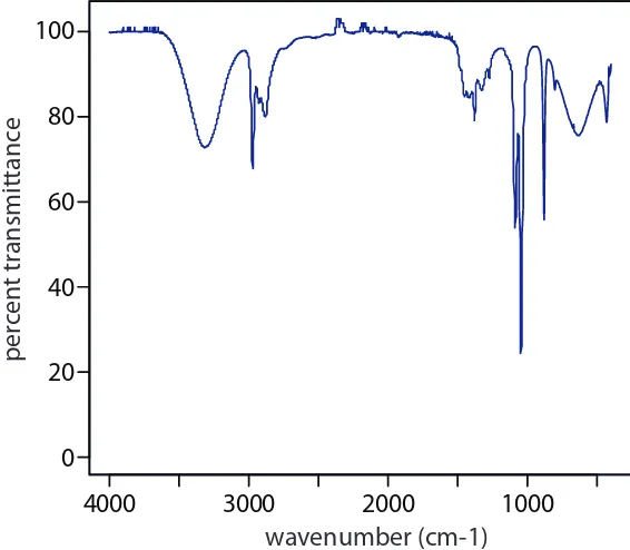
energy of hn0. Transitions in which Dn is ±1 give rise to the fundamental absorption lines. Weaker absorption lines, called overtones, result from transitions in which Dn is ±2 or ±3. he number of possible normal vibra-tional modes for a linear molecule is 3N – 5, and for a non-linear molecule is 3N – 6, where N is the number of atoms in the molecule. Not surprisingly, infrared spectra often show a considerable number of absorption bands. Even a relatively simple molecule, such as ethanol (C2H6O), for example, has 3 � 9 – 6, or 21 possible normal modes of vibration, although not all of these vibrational modes give rise to an absorption. he IR spectrum for ethanol is shown in Figure 10.16.
UV/VIS SPECTRAFOR MOLECULESAND IONS
he valence electrons in organic molecules and polyatomic ions, such as CO32–, occupy quantized sigma bonding, s, pi bonding, p, and non-bond-ing, n, molecular orbitals (MOs). Unoccupied sigma antibondnon-bond-ing, s*, and pi antibonding, p*, molecular orbitals are slightly higher in energy. Because the diference in energy between the highest-energy occupied MOs and
Figure 10.16 Infrared spectrum of ethanol.
Why does a non-linear molecule have 3N – 6 vibrational modes? Consider a molecule of methane, CH4. Each of the ive atoms in methane can move in one of three directions (x, y, and z) for a total of 5 � 3 = 15 diferent ways in which the
molecule can move. A molecule can move in three ways: it can move from one place to another, what we call translational mo-tion; it can rotate around an axis; and its bonds can stretch and bend, what we call vibrational motion.
Because the entire molecule can move in the x, y, and z directions, three of methane’s 15 diferent motions are translational. In addition, the molecule can rotate about its x, y, and z axes, accounting for three additional forms of motion. his leaves 15– 3– 3 = 9 vibrational modes.
A linear molecule, such as CO2, has 3N – 5 vibrational modes because it can rotate around only two axes.
4000 3000 2000 1000
0 20 40 60 80 100
wavenumber (cm-1)
per
cen
t tr
ansmittanc
the lowest-energy unoccupied MOs corresponds to ultraviolet and visible radiation, absorption of a photon is possible.
Four types of transitions between quantized energy levels account for most molecular UV/Vis spectra. Table 10.5 lists the approximate wave-length ranges for these transitions, as well as a partial list of bonds, func-tional groups, or molecules responsible for these transitions. Of these tran-sitions, the most important are n→π∗ and π→π∗ because they involve important functional groups that are characteristic of many analytes and because the wavelengths are easily accessible. he bonds and functional groups that give rise to the absorption of ultraviolet and visible radiation are called chromophores.
Many transition metal ions, such as Cu2+ and Co2+, form colorful solu-tions because the metal ion absorbs visible light. he transisolu-tions giving rise to this absorption are valence electrons in the metal ion’s d-orbitals. For a free metal ion, the ive d-orbitals are of equal energy. In the presence of a complexing ligand or solvent molecule, however, the d-orbitals split into two or more groups that difer in energy. For example, in an octahedral complex of Cu(H2O)62+ the six water molecules perturb the d-orbitals into two groups, as shown in Figure 10.17. he resulting d–d transitions for transition metal ions are relatively weak.
A more important source of UV/Vis absorption for inorganic metal– ligand complexes is charge transfer, in which absorption of a photon pro-duces an excited state in which there is transfer of an electron from the metal, M, to the ligand, L.
M—L + hn (M+—L–)*
Charge-transfer absorption is important because it produces very large ab-sorbances. One important example of a charge-transfer complex is that of o-phenanthroline with Fe2+, the UV/Vis spectrum for which is shown in
Figure 10.18. Charge-transfer absorption in which an electron moves from the ligand to the metal also is possible.
Comparing the IR spectrum in Figure 10.16 to the UV/Vis spectrum in
Figure 10.18 shows us that UV/Vis absorption bands are often signiicantly broader than those for IR absorption. We can use Figure 10.15 to explain
Table 10.5 Electronic Transitions Involving
n
,
s
, and
p
Molecular Orbitals
Transition Wavelength Range Examples
σ→σ∗ <200 nm C–C, C–H
n→σ∗ 160–260 nm H2O, CH3OH, CH3Cl
π→π∗ 200–500 nm C=C, C=O, C=N, C≡C
n→π∗ 250–600 nm C=O, C=N, N=N, N=O
Figure 10.17 Splitting of the d -orbitals in an octahedral ield.
Why is a larger absorbance desirable? An analytical method is more sensitive if a smaller concentration of analyte gives a larger signal.
d
x2–y2d
z2d
xyd
xzd
yzwhy this is true. When a species absorbs UV/Vis radiation, the transition between electronic energy levels may also include a transition between vi-brational energy levels. he result is a number of closely spaced absorption bands that merge together to form a single broad absorption band.
UV/VIS SPECTRAFOR ATOMS
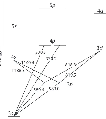
he energy of ultraviolet and visible electromagnetic radiation is suicient to cause a change in an atom’s valence electron coniguration. Sodium, for example, has a single valence electron in its 3s atomic orbital. As shown in Figure 10.19, unoccupied, higher energy atomic orbitals also exist.
Absorption of a photon is accompanied by the excitation of an electron from a lower-energy atomic orbital to an orbital of higher energy. Not all possible transitions between atomic orbitals are allowed. For sodium the only allowed transitions are those in which there is a change of ±1 in the orbital quantum number (l); thus transitions from s p orbitals are allowed, and transitions from s d orbitals are forbidden.
Figure 10.18 UV/Vis spectrum for the metal–ligand complex Fe(phen)32+, where phen is the ligand o -phenanthroline.
Figure 10.19 Valence shell energy level diagram for so-dium. he wavelengths (in wavenumbers) correspond-ing to several transitions are shown.
he valence shell energy level diagram in Figure 10.19 might strike you as odd because it shows that the 3p orbitals are split into two groups of slightly diferent energy. he reasons for this splitting are unimportant in the context of our treat-ment of atomic absorption. For further information about the reasons for this splitting, consult the chapter’s additional resources.
400 450 500 550 600 650 700
0.0 0.2 0.4 0.6 0.8 1.0 1.2
wavelength (nm)
absor
banc
e
1138.3
589.6 589.0 819.5 818.3 330.2
330.3 1140.4
3s
3p
3d
4s
4p
4d
5s
5p
Ener
he atomic absorption spectrum for Na is shown in Figure 10.20, and is typical of that found for most atoms. he most obvious feature of this spectrum is that it consists of a small number of discrete absorption lines corresponding to transitions between the ground state (the 3s atomic or-bital) and the 3p and 4p atomic orbitals. Absorption from excited states, such as the 3p 4s and the 3p 3d transitions included in Figure 10.19, are too weak to detect. Because an excited state’s lifetime is short—typically an excited state atom takes 10–7 to 10–8 s to return to a lower energy state— an atom in the exited state is likely to return to the ground state before it has an opportunity to absorb a photon.
Another feature of the atomic absorption spectrum in Figure 10.20 is the narrow width of the absorption lines, which is a consequence of the ixed diference in energy between the ground and excited states. Natural line widths for atomic absorption, which are governed by the uncertainty principle, are approximately 10–5 nm. Other contributions to broadening increase this line width to approximately 10–3 nm.
10B.2 Transmittance and Absorbance
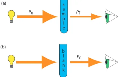
As light passes through a sample, its power decreases as some of it is ab-sorbed. his attenuation of radiation is described quantitatively by two separate, but related terms: transmittance and absorbance. As shown in Figure 10.21a, transmittance is the ratio of the source radiation’s power exiting the sample, PT, to that incident on the sample, P0.
T P
P = T
0
10.1 Multiplying the transmittance by 100 gives the percent transmittance, %T, which varies between 100% (no absorption) and 0% (complete absorp-tion). All methods of detecting photons—including the human eye and modern photoelectric transducers—measure the transmittance of electro-magnetic radiation.
Figure 10.20 Atomic absorption spectrum for sodium. Note that the scale on the x-axis includes a break.
588.5 589.0 589.5 330.0 330.2 330.4
wavelength (nm)
590.0
1.0
0.8
0.6
0.4
0.2
0
absor
banc
e
3s 4p
Equation 10.1 does not distinguish between diferent mechanisms that prevent a photon emitted by the source from reaching the detector. In addi-tion to absorpaddi-tion by the analyte, several addiaddi-tional phenomena contribute to the attenuation of radiation, including relection and absorption by the sample’s container, absorption by other components in the sample’s matrix, and the scattering of radiation. To compensate for this loss of the radiation’s power, we use a method blank. As shown in Figure 10.21b, we redeine P0 as the power exiting the method blank.
An alternative method for expressing the attenuation of electromag-netic radiation is absorbance, A, which we deine as
A T P
P = −log = −log T
0
10.2 Absorbance is the more common unit for expressing the attenuation of radiation because it is a linear function of the analyte’s concentration.
Example 10.3
A sample has a percent transmittance of 50%. What is its absorbance?
S
OLUTIONA percent transmittance of 50.0% is the same as a transmittance of 0.500 Substituting into equation 10.2 gives
A= −logT = −log( .0 500)=0 301.
Figure 10.21 (a) Schematic diagram showing the attenuation of radiation passing through a sample; P0 is the radiant power from the source and PT is the radiant power transmitted by the sample. (b) Schematic diagram showing how we redeine
P0 as the radiant power transmitted by the blank. Redeining P0 in this way cor-rects the transmittance in (a) for the loss of radiation due to scattering, relection, or absorption by the sample’s container and absorption by the sample’s matrix.
We will show that this is true in Section 10B.3.
Practice Exercise 10.3
What is the %T for a sample if its absorbance is 1.27? Click here to review your answer to this exercise.
b
l
a
n
k
P0 (b)
s
a
m
p
l
e
P0 PT
Equation 10.1 has an important consequence for atomic absorption. As we saw in Figure 10.20, atomic absorption lines are very narrow. Even with a high quality monochromator, the efective bandwidth for a continuum source is 100–1000� greater than the width of an atomic absorption line. As a result, little of the radiation from a continuum source is absorbed (P0 ≈ PT), and the measured absorbance is efectively zero. For this reason, atomic
absorption requires a line source instead of a continuum source. 10B.3 Absorbance and Concentration: Beer’s Law
When monochromatic electromagnetic radiation passes through an inini-tesimally thin layer of sample of thickness dx, it experiences a decrease in its power of dP (Figure 10.22). he fractional decrease in power is propor-tional to the sample’s thickness and the analyte’s concentration, C; thus
−dP =
P αCdx 10.3
where P is the power incident on the thin layer of sample, and a is a pro-portionality constant. Integrating the left side of equation 10.3 over the entire sample
−
∫
dP =∫
P C dx
P P
o b
0 T
α
ln P
P bC
0 T
= α
converting from ln to log, and substituting in equation 10.2, gives
A=abC 10.4
where a is the analyte’s absorptivity with units of cm–1 conc–1. If we ex-press the concentration using molarity, then we replace a with the molar absorptivity, e, which has units of cm–1 M–1.
A= εbC 10.5
he absorptivity and molar absorptivity are proportional to the probability that the analyte absorbs a photon of a given energy. As a result, values for both a and e depend on the wavelength of the absorbed photon.
Figure 10.22 Factors used in deriving the Beer-Lambert law.
dx
x = 0
x = b
Example 10.4
A 5.00 � 10–4 M solution of an analyte is placed in a sample cell with a pathlength of 1.00 cm. When measured at a wavelength of 490 nm, the solution’s absorbance is 0.338. What is the analyte’s molar absorptivity at this wavelength?
S
OLUTIONSolving equation 10.5 for e and making appropriate substitutions gives ε = =
× − =
− A
bC
0 338
1 00 10 4 676
1
.
( . cm)(5.00 M) cm MM
−1
Practice Exercise 10.4
A solution of the analyte from Example 10.4 has an absorbance of 0.228 in a 1.00-cm sample cell. What is the analyte’s concentration?
Click here to review your answer to this exercise.
Equation 10.4 and equation 10.5, which establish the linear relation-ship between absorbance and concentration, are known as the Beer-Lam-bert law, or more commonly, as beer’s law. Calibration curves based on Beer’s law are common in quantitative analyses.
10B.4 Beer’s Law and Multicomponent Samples
We can extend Beer’s law to a sample containing several absorbing compo-nents. If there are no interactions between the components, the individual absorbances, Ai, are additive. For a two-component mixture of analyte’s X and Y, the total absorbance, Atot, is
Atot =AX+AY =εXbCX+εYbCY
Generalizing, the absorbance for a mixture of n components, Amix, is
A Ai bC
i n
i i
i n
mix = =
= =
∑
∑
1 1
ε 10.6
10B.5 Limitations to Beer’s Law
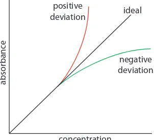
Beer’s law suggests that a calibration curve is a straight line with a y-inter-cept of zero and a slope of ab or eb. In many cases a calibration curve devi-ates from this ideal behavior (Figure 10.23). Deviations from linearity are divided into three categories: fundamental, chemical, and instrumental.
FUNDAMENTAL LIMITATIONSTO BEER’S LAW
Beer’s law is a limiting law that is valid only for low concentrations of analyte. here are two contributions to this fundamental limitation to Beer’s law. At Figure 10.23 Calibration curves
show-ing positive and negative deviations from the ideal Beer’s law calibration curve, which is a straight line.
ideal
negative deviation positive
deviation
concentration
absor
banc
higher concentrations the individual particles of analyte no longer behave independently of each other. he resulting interaction between particles of analyte may change the analyte’s absorptivity. A second contribution is that the analyte’s absorptivity depends on the sample’s refractive index. Because the refractive index varies with the analyte’s concentration, the values of a and e may change. For suiciently low concentrations of analyte, the refrac-tive index is essentially constant and the calibration curve is linear.
CHEMICAL LIMITATIONSTO BEER’S LAW
A chemical deviation from Beer’s law may occur if the analyte is involved in an equilibrium reaction. Consider, as an example, an analysis for the weak acid, HA. To construct a Beer’s law calibration curve we prepare a series of standards—each containing a known total concentration of HA—and measure each standard’s absorbance at the same wavelength. Because HA is a weak acid, it is in equilibrium with its conjugate weak base, A–.
HA(aq)+H O2 ( )l H O3 +(aq)+A−(aq)
If both HA and A– absorb at the chosen wavelength, then Beer’s law is
A=εHAbCHA+εAbCA 10.7
where CHA and CA are the equilibrium concentrations of HA and A–. Be-cause the weak acid’s total concentration, Ctotal, is
Ctotal =CHA+CA
the concentrations of HA and A– can be written as
CHA= αHACtotal 10.8
CA = −(1 αHA)Ctotal 10.9
where aHA is the fraction of weak acid present as HA. Substituting equation 10.8 and equation 10.9 into equation 10.7 and rearranging, gives
A=(ε αHA HA+εA−ε αA HA)bCtotal 10.10 To obtain a linear Beer’s law calibration curve, one of two conditions must be met. If aHA and aA have the same value at the chosen wavelength, then equation 10.10 simpliies to
A= εAbCtotal
Alternatively, if aHA has the same value for all standards, then each term within the parentheses of equation 10.10 is constant—which we replace with k—and a linear calibration curve is obtained at any wavelength.
Because HA is a weak acid, the value of aHA varies with pH. To hold
aHA constant we bufer each standard to the same pH. Depending on the relative values of aHA and aA, the calibration curve has a positive or a negative deviation from Beer’s law if we do not bufer the standards to the same pH.
INSTRUMENTAL LIMITATIONSTO BEER’S LAW
here are two principal instrumental limitations to Beer’s law. he irst limi-tation is that Beer’s law assumes that the radiation reaching the sample is of a single wavelength—that is, that the radiation is purely monochromatic. As shown in Figure 10.10, however, even the best wavelength selector passes radiation with a small, but inite efective bandwidth. Polychromatic ra-diation always gives a negative deviation from Beer’s law, but the efect is smaller if the value of e is essentially constant over the wavelength range passed by the wavelength selector. For this reason, as shown in Figure 10.24, it is better to make absorbance measurements at the top of a broad absorp-tion peak. In addiabsorp-tion, the deviaabsorp-tion from Beer’s law is less serious if the source’s efective bandwidth is less than one-tenth of the natural bandwidth of the absorbing species.5 When measurements must be made on a slope,
linearity is improved by using a narrower efective bandwidth.
Stray radiation is the second contribution to instrumental deviations from Beer’s law. Stray radiation arises from imperfections in the wavelength selector that allow light to enter the instrument and reach the detector without passing through the sample. Stray radiation adds an additional contribution, Pstray, to the radiant power reaching the detector; thus
A P P
P P
= − +
+ log T stray
0 stray
For a small concentration of analyte, Pstray is signiicantly smaller than P0 and PT, and the absorbance is unafected by the stray radiation. At a higher concentration of analyte, however, less light passes through the sample and
5 (a) Strong, F. C., III Anal. Chem.1984, 56, 16A–34A; Gilbert, D. D. J. Chem. Educ.1991, 68, A278–A281.
For a monoprotic weak acid, the equation for aHA is
αHA 3
3 a H O H O = + + + [ ]
[ ] K
Problem 10.6 in the end of chapter prob-lems asks you to explore this chemical limitation to Beer’s law.
Figure 10.24 Efect of the choice of wavelength on the linearity of a Beer’s law calibration curve.
Another reason for measuring absorbance at the top of an absorbance peak is that it provides for a more sensitive analysis. Note that the green calibration curve in Figure 10.24 has a steeper slope—a greater sensitivity—than the red calibra-tion curve.
Problem 10.7 in the end of chapter prob-lems ask you to explore the efect of poly-chromatic radiation on the linearity of Beer’s law.
PT and Pstray may be similar in magnitude. his results is an absorbance that is smaller than expected, and a negative deviation from Beer’s law.
10C UV/Vis and IR Spectroscopy
In Figure 10.9 we examined Nessler’s original method for matching the color of a sample to the color of a standard. Matching the colors was a labor intensive process for the analyst. Not surprisingly, spectroscopic methods of analysis were slow to develop. he 1930s and 1940s saw the introduction of photoelectric transducers for ultraviolet and visible radiation, and ther-mocouples for infrared radiation. As a result, modern instrumentation for absorption spectroscopy became routinely available in the 1940s—progress has been rapid ever since.
10C.1 Instrumentation
Frequently an analyst must select—from among several instruments of dif-ferent design—the one instrument best suited for a particular analysis. In this section we examine several diferent instruments for molecular absorp-tion spectroscopy, emphasizing their advantages and limitaabsorp-tions. Methods of sample introduction are also covered in this section.
INSTRUMENT DESIGNSFOR MOLECULAR UV/VIS ABSORPTION
Filter Photometer. he simplest instrument for molecular UV/Vis
absorp-tion is a filter photometer (Figure 10.25), which uses an absorpabsorp-tion or interference ilter to isolate a band of radiation. he ilter is placed between the source and the sample to prevent the sample from decomposing when exposed to higher energy radiation. A ilter photometer has a single optical path between the source and detector, and is called a single-beam instru-ment. he instrument is calibrated to 0% T while using a shutter to block the source radiation from the detector. After opening the shutter, the
in-Problem 10.8 in the end of chapter prob-lems ask you to explore the efect of stray radiation on the linearity of Beer’s law.
Figure 10.25 Schematic diagram of a ilter photom-eter. he analyst either inserts a removable ilter or the ilters are placed in a carousel, an example of which is shown in the photographic inset. he analyst selects a ilter by rotating it into place.
he percent transmittance varies between 0% and 100%. As we learned in Figure 10.21, we use a blank to determine P0,
which corresponds to 100% T. Even in the absence of light the detector records a sig-nal. Closing the shutter allows us to assign 0% T to this signal. Together, setting 0% T and 100% T calibrates the instrument. he amount of light passing through a sample produces a signal that is greater than or equal to that for 0% T and smaller than or equal to that for 100%T.
s
a
m
p
l
e
b
l
a
n
k
open
closed source
detector
filter shutter
strument is calibrated to 100% T using an appropriate blank. he blank is then replaced with the sample and its transmittance measured. Because the source’s incident power and the sensitivity of the detector vary with wave-length, the photometer must be recalibrated whenever the ilter is changed. Photometers have the advantage of being relatively inexpensive, rugged, and easy to maintain. Another advantage of a photometer is its portability, making it easy to take into the ield. Disadvantages of a photometer include the inability to record an absorption spectrum and the source’s relatively large efective bandwidth, which limits the calibration curve’s linearity.
Single-Beam Spectrophotometer. An instrument that uses a
monochro-mator for wavelength selection is called a spectrophotometer. he simplest spectrophotometer is a single-beam instrument equipped with a ixed-wavelength monochromator (Figure 10.26). Single-beam spectro-photometers are calibrated and used in the same manner as a photometer. One example of a single-beam spectrophotometer is hermo Scientiic’s Spectronic 20D+, which is shown in the photographic insert to Figure 10.26. he Spectronic 20D+ has a range of 340–625 nm (950 nm when using a red-sensitive detector), and a ixed efective bandwidth of 20 nm. Battery-operated, hand-held single-beam spectrophotometers are available, which are easy to transport into the ield. Other single-beam spectropho-tometers also are available with efective bandwidths of 2–8 nm. Fixed wavelength single-beam spectrophotometers are not practical for recording spectra because manually adjusting the wavelength and recalibrating the spectrophotometer is awkward and time-consuming. he accuracy of a single-beam spectrophotometer is limited by the stability of its source and detector over time.
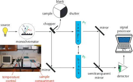
Double-Beam Spectrophotometer. he limitations of ixed-wavelength,
single-beam spectrophotometers are minimized by using a double-beam spectrophotometer (Figure 10.27). A chopper controls the radiation’s path, Figure 10.26 Schematic diagram of a ixed-wavelength
single-beam spectrophotometer. he photographic in-set shows a typical instrument. he shutter remains closed until the sample or blank is placed in the sample compartment. he analyst manually selects the wave-length by adjusting the wavewave-length dial. Inset photo modiied from: Adi (www.commons.wikipedia.org).
λ1λ2
λ3
s
a
m
p
l
e
b
l
a
n
k
open
closed shutter source
monochromator
detector
signal processor
wavelength dial sample
compartment
0% T and 100% T adjustment
P0
alternating it between the sample, the blank, and a shutter. he signal processor uses the chopper’s known speed of rotation to resolve the signal reaching the detector into the transmission of the blank, P0, and the sample, PT. By including an opaque surface as a shutter, it is possible to
continu-ously adjust 0% T. he efective bandwidth of a double-beam spectropho-tometer is controlled by adjusting the monochromator’s entrance and exit slits. Efective bandwidths of 0.2–3.0 nm are common. A scanning mono-chromator allows for the automated recording of spectra. Double-beam instruments are more versatile than single-beam instruments, being useful for both quantitative and qualitative analyses, but also are more expensive.
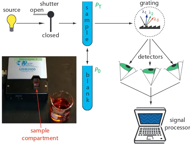
Diode Array Spectrometer. An instrument with a single detector can
monitor only one wavelength at a time. If we replace a single photomul-tiplier with many photodiodes, we can use the resulting array of detectors to record an entire spectrum simultaneously in as little as 0.1 s. In a diode array spectrometer the source radiation passes through the sample and is dispersed by a grating (Figure 10.28). he photodiode array is situated at the grating’s focal plane, with each diode recording the radiant power over a narrow range of wavelengths. Because we replace a full monochromator with just a grating, a diode array spectrometer is small and compact.
Figure 10.27 Schematic diagram of a scanning, double-beam spectrophotometer. A chopper directs the source’s radiation, using a transparent window to pass radiation to the sample and a mirror to relect radiation to the blank. he chopper’s opaque surface serves as a shutter, which allows for a constant adjustment of the spectro-photometer’s 0% T. he photographic insert shows a typical instrument. he unit in the middle of the photo is a temperature control unit that allows the sample to be heated or cooled.
λ1 λ2
λ3
s
a
m
p
l
e
source
monochromator
detector
b
l
a
n
k
signal processor chopper
mirror
mirror
semitransparent mirror sample
blank
shutter
sample compartment temperature
control
One advantage of a diode array spectrometer is the speed of data acqui-sition, which allows to collect several spectra for a single sample. Individual spectra are added and averaged to obtain the inal spectrum. his signal averaging improves a spectrum’s signal-to-noise ratio. If we add together n spectra, the sum of the signal at any point, x, increases as nSx, where Sx is the signal. he noise at any point, Nx, is a random event, which increases as
nNx when we add together n spectra. he signal-to-noise ratio (S/N) after n scans is
S N nS nN n S N x x x x = =
where Sx/Nx is the signal-to-noise ratio for a single scan. he impact of sig-nal averaging is shown in Figure 10.29. he irst spectrum shows the sigsig-nal for a single scan, which consists of a single, noisy peak. Signal averaging using 4 scans and 16 scans decreases the noise and improves the signal-to-noise ratio. One disadvantage of a photodiode array is that the efective bandwidth per diode is roughly an order of magnitude larger than that for a high quality monochromator.
Sample Cells. he sample compartment provides a light-tight environment
that limits the addition of stray radiation. Samples are normally in the liquid or solution state, and are placed in cells constructed with UV/Vis transparent materials, such as quartz, glass, and plastic (Figure 10.30). A quartz or fused-silica cell is required when working at a wavelength <300 nm where other materials show a signiicant absorption. he most common pathlength is 1 cm (10 mm), although cells with shorter (as little as 0.1 cm) and longer pathlengths (up to 10 cm) are available. Longer pathlength cells Figure 10.29 Efect of signal averaging
on a spectrum’s signal-to-noise ratio. From top to bottom: spectrum for a single scan; average spectrum after four scans; and average spectrum after adding 16 scans.
λ1 λ2 λ3 s a m p l e b l a n k open closed shutter source grating detectors signal processor sample compartment P0 PT
Figure 10.28 Schematic diagram of a diode array spectrophotometer. he photographic in-sert shows a typical instrument. Note that the 50-mL beaker provides a sense of scale.
500 550 600 650 700
wavelength 1.0 0.8 0.6 0.4 0.2 0 absor banc e 1 scan
500 550 600 650 700
wavelength 1.0 0.8 0.6 0.4 0.2 0 absor banc e 4 scans
500 550 600 650 700
are useful when analyzing a very dilute solution, or for gas samples. he highest quality cells allow the radiation to strike a lat surface at a 90o angle, minimizing the loss of radiation to relection. A test tube is often used as a sample cell with simple, single-beam instruments, although diferences in the cell’s pathlength and optical properties add an additional source of error to the analysis.
If we need to monitor an analyte’s concentration over time, it may not be possible to physically remove samples for analysis. his is often the case, for example, when monitoring industrial production lines or waste lines, when monitoring a patient’s blood, or when monitoring environmental systems. With a fiber-optic probe we can analyze samples in situ. An ex-ample of a remote sensing iber-optic probe is shown in Figure 10.31. he probe consists of two bundles of iber-optic cable. One bundle transmits radiation from the source to the probe’s tip, which is designed to allow the sample to low through the sample cell. Radiation from the source passes through the solution and is relected back by a mirror. he second bundle
Figure 10.30 Examples of sample cells for UV/Vis spectroscopy. From left to right (with path lengths in pa-rentheses): rectangular plastic cuvette (10.0 mm), rectangular quartz cuvette (5.000 mm), rectangular quartz cuvette (1.000 mm), cylindrical quartz cuvette (10.00 mm), cylindrical quartz cuvette (100.0 mm). Cells often are available as a matched pair, which is important when using a double-beam instrument.
Figure 10.31 Example of a iber-optic probe. he inset photographs provide a close-up look at the probe’s low cell and the relecting mirror
light in light out
probe’s tip reflecting
mirror
of iber-optic cable transmits the nonabsorbed radiation to the wavelength selector. Another design replaces the low cell shown in Figure 10.31 with a membrane containing a reagent that reacts with the analyte. When the analyte difuses across the membrane it reacts with the reagent, producing a product that absorbs UV or visible radiation. he nonabsorbed radiation from the source is relected or scattered back to the detector. Fiber optic probes that show chemical selectivity are called optrodes.6
INSTRUMENT DESIGNSFOR INFRARED ABSORPTION
Filter Photometer. he simplest instrument for IR absorption spectroscopy
is a ilter photometer similar to that shown in Figure 10.25 for UV/Vis ab-sorption. hese instruments have the advantage of portability, and typically are used as dedicated analyzers for gases such as HCN and CO.
Double-beam spectrophotometer. Infrared instruments using a
mono-chromator for wavelength selection use double-beam optics similar to tha