*Corresponding author.
Duration dependence and nonparametric
heterogeneity: A Monte Carlo study
Michael Baker, Angelo Melino
*
Department of Economics, University of Toronto, 150 St. George St., Toronto, Ont., Canada M5S 3G7
Received 1 December 1997; received in revised form 1 June 1999
Abstract
We examine the behaviour of the nonparametric maximum likelihood estimator (NPMLE) for a discrete duration model with unobserved heterogeneity and unknown duration dependence. We"nd that a nonparametric speci"cation of either the duration dependence or unobserved heterogeneity, when the other feature of the hazard is known to be absent, leads to estimators that are well behaved even in modestly sized samples. In contrast, there is a large and systematic bias in the parameters of these components when both are speci"ed nonparametrically, as well as a complementary bias in the coe$cients on observed heterogeneity. Furthermore, these biases diminish very gradually as sample size increases. We"nd that a minor modi"cation of the quasilikelihood that penalizes speci"cations with many points of support leads to a dramatic improvement. ( 2000 Elsevier Science S.A. All rights reserved.
Keywords: NPMLE; Discrete duration model
1. Introduction
Hazard models of event durations"nd application in many areas of applied economics ranging from the analysis of unemployment spells to studies of fecundity. There is now widespread acknowledgment that inference in these models can be subject to speci"cation error from a number of sources. One
cause is unobserved heterogeneity arising from the omission of (possibly unob-servable) variables that a!ect the hazard. A common antidote to this problem is to model the unobserved heterogeneity as individual-speci"c random e!ects. There is growing recognition, however, that inference can be sensitive to the assumed distribution of the unobserved heterogeneity. This issue is of particular importance when the hazard (the conditional probability of exit) exhibits dura-tion dependence. As in many other areas of econometrics, nonparametric approaches have been proposed in the absence of any guidance from economic theory about functional form. In hazard models, the nonparametric approach has been applied with some success to both the speci"cation of the baseline hazard (e.g., Ham and Rea, 1987; Meyer, 1990) and the distribution of unobser-ved individual e!ects (e.g., Nickell, 1979; Heckman and Singer, 1984).
Empirical researchers increasingly take heed of these results, but compro-mises are made. For example, semiparametric models, that is models made up of a mixture of parametric and nonparametric components, are often used. Typi-cally, the hazard is characterized by a parametric form, but either the duration dependence or the unobserved heterogeneity distribution is modelled non-parametrically. While there is an obvious argument to be #exible in both dimensions, numerical di$culties often hinder the estimation of models with nonparametric speci"cations of both the baseline hazard and the unobserved heterogeneity (e.g., Meyer, 1990; Baker and Rea, 1998). In fact, largely in response to computational problems, the nonparametric estimators of either component are often only partially adopted. For example, the nonparametric maximum likelihood estimator (NPMLE) of the unobserved heterogeneity distribution proposed by Heckman and Singer (1984) in e!ect assumes that the unobserved random e!ects are drawn from a discrete distribution with unknown support and an unknown number of mass points. In many studies, the number of mass points is simply speci"ed a priori as at most two, or the search for additional mass points is abandoned when numerical problems are encountered. Similar compromises are made in the speci"cation of the duration dependence. In a common nonparametric approach, the baseline hazard is speci"ed as a step function. Therefore, the width of the steps must be chosen. Narrow steps will allow for very#exible shapes for the duration dependence but may require enormous amounts of data for reliable estimation. In practice there appears to be a trade-o!between widening the step (and thus imposing more parametric structure on the duration dependence) and relaxing the speci"cation of the unobserved e!ects (e.g., Narendranathan and Stewart, 1993), so re-searchers must decide which of these two features to emphasize.
We begin by outlining a computational strategy for the NPMLE with unobserved heterogeneity. This is a more familiar formulation of the strategy due to Lindsay (1983) that was adapted by Heckman and Singer (1984), and provides a systematic approach to determining the location and number of mass points for the heterogeneity distribution. We next provide Monte Carlo evid-ence on the behaviour of the NPMLE in a variety of environments. Both the data generating process (DGP) used to construct the sample data, and the quasi-likelihood (QL) speci"cation used for estimation, vary across the experi-ments. The latter di!er by the speci"cation of the time functions used to model the true duration dependence. To anticipate our main results, we "nd that a nonparametric speci"cation for either the duration dependence or unobserved heterogeneity, when the other feature of the hazard is known to be absent, leads to estimators that are well behaved even in modestly sized samples. However, the combination of a #exible speci"cation for both duration dependence and unobserved heterogeneity leads to a very reliable and systematic bias. The estimated time functions are biased toward"nding positive duration depend-ence and the NPMLE overestimates the dispersion of the random e!ects. Often both duration dependence and unobserved heterogeneity are of secondary interest, so it is important to emphasize that these faults lead to a large and signi"cant bias for the parameters on observed heterogeneity, which we will refer to as b. It is well known that ignoring unobserved heterogeneity, even though it is independent of observed heterogeneity, biasesbtowards zero. It is perhaps not surprising that we"nd the exaggerated dispersion in the estimated heterogeneity distribution coincides with a bias inbaway from zero. Moreover, the bias is extremely large and goes away very slowly even as the sample grows to sizes that are enormous by today's standards. It appears that the poor sampling performance of the NPMLE of unobserved heterogeneity stems al-most entirely from the fact that it"nds too many&spurious'points of support. A minor modi"cation of the QL to include a term that penalizes speci"cations with many points of support (for example, the Schwartz or Hannan-Quinn Information Criterion) seems like a natural solution, and was proposed in a similiar setting by Leroux (1992). We"nd that the penalized NPMLE leads to a dramatic improvement in the sampling properties of the various estimators and a much more reliable estimator forb.
2. A computational strategy
1While this is essentially the incremental strategy adopted in some studies in the area, in practice it can be problematic if the location of the additional mass point is&poorly'chosen. Our point in this section is to suggest a systematic approach to identifying the location of additional points of support. An alternative strategy would be to estimate the model using a grid of values for thehiover a&reasonable'range. See for example Lemieux and MacLeod (1995).
is based in introspection (we developed the algorithm independently before "nding it in the cited studies); the observation that estimation strategies adopted by many researchers in this area are essentially ad hoc; and, numerous conversa-tions with researchers. Our presentation avoids the Gateaux di!erential used by Heckman and Singer and replaces it with the more familiar Kuhn}Tucker multiplier.
Assume that heterogeneity is indexed by a single parameterh, which is known to lie in the interval [hL, hH]. Let ¸
ih,¸h(a,hi) denote the likelihood for individual h given the heterogeneity parameter takes on the value h
i, where
a3Rpare other parameters. Suppose that the heterogeneity parameter is dis-tributed as a discrete random variable withNh points of support. The loglikeli-hood for the individual is
where the probability weights satisfy+P
i"1 andPi*0. The loglikelihood for
The parameters of the heterogeneity distribution areNh(the number of points of support), along with (h
i,Pi; i"1,2,Nh). We proceed assuming that these
parameters are functionally independent of a. Given that Nh is an integer, a sensible strategy is to pick a value for the number of points of support, say
NM h, estimate the remaining parameters and then check if the likelihood can be increased by adding an additional point of support to the distribution ofh.1
Suppose we have the MLE Ma(, hKi,PKi; i"1,2, NM hN, conditional on the
assumption that there are NM h points of support. Let hM be a candidate for an additional point of support. Our approach is to consider the optimal values of (P
1,2,PNMh`1), "xing a"a(,hi"hKi for i"1,2,Nh and hNMh`1"hM. If the
optimal value ofP
NMh`1"0, then adding a point of support athM cannot increase
the sample likelihood. If this is true for allhM3[hL, hH] then we have found the NPMLE. If instead the optimal value of P
NMh`1'0, then it is possible to
Formally we can write the problem as
Notice that the objective function is concave in MP
iN and the constraints are linear, so the optimum is characterized by the Kuhn}Tucker "rst-order conditions:
It is not possible to solve for the optimal probabilities in closed form from the "rst-order conditions, but we can use them to evaluate a particular candidate. First, multiply (2.4) by P
i, sum over i, and use Eqs. (2.5) and (2.6) to obtain
j"!N
h. Substituting back into (2.4) we eliminatej, and obtain
k MPK iNmaximize the likelihood forNMh points of support, it is easy to show that
k
iwill be zero fori"1,2, NM h(the right-hand side of (2.7) is just the gradient of the loglikelihood (2.2) with respect to these probabilities). Ifk
NMh`1*0 then the
"rst-order conditions are satis"ed at the candidate probabilities so the likeli-hood cannot be improved by adding a point of support athM. If this is true for all
hM3[hL,hH] then we have found the NPMLE. If, on the other hand,k
NMh`1(0
for some choice of hM, then the candidate probabilities violate the "rst-order conditions and it is possible to increase the sample likelihood by adding a point of support athM.
Heckman and Singer (1984) show that the (negative of the) Kuhn}Tucker multipliers given by (2.7) are Gateaux derivatives, and a necessary and su$cient condition for the NPMLE (using our notation) isk
NMh`1*0 for allhM3[hL, hH].
This result suggests the following algorithm:
Step 0: SetNM h"1 andP
1"1. Choose initial values foraandh1.
Step 1: Given the current value ofNM h, maximize the likelihood overaand
2It is not numerically possible to achieve a gradient of the log-likelihood that is exactly zero, but we found that Step 2 can be sensitive to even very small errors in computing the optimal probabilities. After a good deal of experimenting, we concluded (at least in our implementation) that inserting an extra step to &polish'the estimated probabilities had no noticeable impact on the parameter estimates but it improved the numerical robustness of our code. In those cases where a point of support was dropped or we achieved even a modest increase in the loglikelihood, we returned immediately to Step 1.
Step 3: Solve (2.3) numerically to obtain new initial values for the probabilities.
Increase the value ofNM h by 1. Return to Step 1.
In our application, the QL is concave in the parameters (a,h), so the initial values chosen in Step 0 can be arbitrary. The problem solved in Step 3 is also very well behaved; we use the reduced gradient method described in Luenberger (1984, Chapter 11). With more than one point of support, Step 1 is the most time consuming and di$cult due to the vagaries of nonlinear estima-tion. We used a modi"ed Newton}Raphson algorithm, but the "nite mixture literature often relies on the EM algorithm (see Lancaster, 1990, Chapter 8). Step 2 appears to work reasonably well in practice (but see Section 6.3 for a suggested improvement).
The algorithm guarantees that the likelihood will increase each time a point of support is added. Heckman and Singer (1984) describe a strategy for choosing [hL,hH] in a systematic way that must include any additional point of support that can increase the QL. We were unable to implement their suggestion. Instead, we chose this interval implicitly so that the probability of exit in the"rst period for all types was restricted to the set [e, 1!e]. Initially, we seteto 10~5, but this value was decreased adaptively if the estimated points of support approached a boundary.
3Campolieti (1997) uses a Dirichlet process prior to construct an estimator that is e!ectively nonparametric but amenable to standard Bayesian inferential techniques in"nite samples.
3. Related research
Although duration data used in economic applications are always reported in discrete units (e.g., days or weeks) and are therefore integer valued, the econo-metric literature is dominated by continuous-time duration models in which the durations can take on all values on the positive real line. In particular, many theoretical and applied studies adopt the mixed proportional hazard model (MPH). The leading special case of the MPH has an instanteous hazard rate of the form
j
ht"exp(Xhb#f(t)#hh) (3.1)
where the three components in (3.1) represent observed heterogeneity, duration dependence, and unobserved heterogeneity, respectively.hhis assumed to be an i.i.d. draw from some unknown distribution that must be estimated along with
band the parameters of the baseline hazard exp(f(t)).
Several analytical results are known for the MPH model. Invoking fairly general assumptions, Elbers and Ridder (1982) showed that the parameters of the MPH model are identi"ed (but see Ridder (1990) and Ishwaran (1996)), and Heckman and Singer (1984) proved that the NPMLE is consistent. The asymp-totic distribution of the NPMLE for this model is not yet known, but Hahn (1994) and Ishwaran (1996) show that, at least for a leading special case, it is not
Jnconsistent.3
4We can show that if the duration dependence function is known to be constant for the"rst two periods, then the model is identi"ed for general mixtures.
proportional hazard model. They also restrict attention to a one-parameter model for duration dependence. They"nd that the NPMLE works reasonably well although there appears to be a small sample advantage to their alternative estimators.
The discrete duration model that we investigate in this paper has been used by many authors. We suspect that this model should lead to estimates with properties that are very similiar to those of the MPH. We know of no analytical results for this model, however, and comparisons of our results with Monte Carlo results for the MPH model can be viewed at best as suggestive.
Closely related to our discrete duration model is the literature on binary choice. Because it is an index model, the results of Cosslett (1983) can be used to show that the regression coe$cients in our discrete duration model are identi-"ed at least up to scale, even if we allow the exit probabilites to vary freely with duration. Cameron and Heckman (1998) provide identi"cation results for a gen-eral class of discrete duration models. They show that identi"cation is enhanced if the index varies with duration. If the index is constant, as is the case in our model, then identi"cation is delicate and requires some additional structure on the transition probabilities. Because it has a discrete factor structure, their Theorem 4 shows that our model is identi"ed, at least if we restrict attention to "nite mixture distributions. We have been unable to extend their results to the general case.4
Finally, there is a large statistical literature on the estimation of mixing distributions (see Lindsay and Lesperance (1995) for a recent survey). While relevant and suggestive, much of this literature is di$cult to adapt to our setting because it excludes the case where there are other parameters of interest. In econometric applications, the main interest is often in the parametersathat are implicit in (2.1). Of course, it is possible that the MLE estimates of amay be e$cient and asymptotically normal even though these properties do not extend to the estimated mixing distribution (Van der Vaart, 1996).
4. Sample design
5These estimates are constructed assuming 4.3 weeks per month. Meyer (1990) reports that the empirical hazards for the"rst four weeks of insured spells in the US are 0.082, 0.066, 0.056, and 0.061. for the period 1978}1983.
6The discrete time hazard is one minus the continuation function.
7All the random numbers were generated using IMSL routines DRNUNF and DRNGAM. We used the multiplier 950706376 and shu%ing.
4.1. DGPs
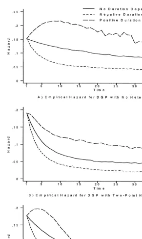
In calibrating our DGP, we tried to choose true hazards that resembled those typically observed in data on unemployment spells, measured in weeks. Ham and Rea (1987) report empirical hazards of 0.171, 0.170, 0.098 and 0.066 for the"rst four weeks of UI insured unemployment spells in Canada, at a time when most spells were insured. Sider (1985) estimates that the continuation probability out of the"rst month of unemployment ranged from 0.41 to 0.59 in the US over the period 1969}1982. This implies (constant) weekly hazards over the"rst month of unemployment ranging from 0.12 to 0.19.5These estimates provide some room for choice. As a benchmark, we tried to generate hazards with the probability of exiting in the"rst period equal to about 0.15, with about half the sample exiting by the fourth week, and that were declining with duration.
We assumed that the probability that a given observationhin our sample survived from time t!1 to time t, hereafter referred to as the continuation
function,6was of the logistic form, that is
S
where the index is of the form
z
ht"Xhb#f(t)#hh. (4.2)
8Using the data from Baker and Rea (1998), theR2for log duration of weekly unemployment spells is about 0.05.
4.1.1. Observed heterogeneity
Because of computational costs, we only considered the case where observed heterogeneity is summarized by a scalar. To ease interpretation and without loss of generality, we setb"1 in all our simulations. Many authors have warned that various properties of estimators can be hidden in a design that considers only symmetric distributions for X. Nonetheless, it is also useful to maintain comparability with previous studies, so we followed Heckman and Singer (1984), Ridder (1987), and Huh and Sickles (1994) and assumed thatX&NID(0,p2
x).
Setting E(X)"0 is a useful normalization that clari"es the interpretation of the remaining parameters. The choice ofp2
x is less obvious. The value ofp2x deter-mines the relative importance of observable heterogeneity and is a key determi-nant in practice of not only how accurately we can estimatebbut whether or not we can distinguish duration dependence from unobserved heterogeneity. One way to choose this parameter is to try to match theR2from a regression of the log of duration on X to values typically observed. On this basis, we chose
p2
x"0.25. This put the averageR2in our DGP with no duration dependence
and no unobserved heterogeneity at about 0.08. Moreover, this value for
p2
x more or less kept the averageR2in all of our DGPs described below in the range 0.05}0.10.8
4.1.2. Duration dependence
We considered three forms for the true duration dependence: none, negative duration dependence, and positive duration dependence. Settingf(t),0 allows us to gauge the e$ciency loss that comes from trying to allow for duration dependence when none is present. The case where, other things equal, the hazard is declining with duration is called negative duration dependence. Of course, a declining hazard is equivalent to a rising continuation function, so that in our parameterization negative duration dependence is associated with anincreasing
path forf(t). We model negative duration dependence by setting
f(t)"1!exp
A
1!t5
B
. (4.3)9None of the estimators that we consider in this paper deal with the possibility that the unobserved heterogeneity may be correlated withX, but it is easy to see what the consequences of such correlation would be in one special case. Suppose we model unobserved heterogeneity as
hI"h#jX, wherehis a random e!ect. This model can be mapped into our set-up by rede"ning the coe$cient onXasbI"b#j.
10Our designs set Var(h)/Var(bX) to 0 or 4 depending on whether or not we have unobserved heterogeneity in the true DGP. In Section 6, we report some results where this ratio is 1. Our results do not appear sensitive to the value of this ratio, but we had no idea what a sensible value would be. We would like to thank a referee for bringing to our attention that Lancaster (1979) using a continuous-time model reports a ratio of 0.5.
4.1.3. Unobserved heterogeneity
We assumed that the unobserved heterogeneity parameterh
h was a random draw from a given distribution.9 We considered three cases: a degenerate distribution (that is, no unobserved heterogeneity); a discrete distribution with two points of support; and a (translated) gamma distribution. In the case of no unobserved heterogeneity, we simply seth
h"1.8. This value was chosen so that
the unconditional probability of exiting at timet"1 was about 0.15. For the discrete distribution, we assumed that each of the two points was equally likely. We set the mean to 1.8 and the variance to unity. This uniquely determined the points of support ath"0.8 andh"2.8. The gamma distribution is often used to model heterogeneity in continuous time hazard models. In contrast to the previous choices, it has a density and the distribution is not symmetric about the mean. We"rst tried to draw gamma random variables from a distribution with mean 1.8 and variance 1, matching the same two moments as in our discrete heterogeneity distribution case. However, we were unhappy with the resulting hazard shapes. After some experimentation, we "rst drew h1
h from a gamma distribution with mean 0.5 and variance 1, and then constructed h
h"
h1
h#1.3.10
4.2. Quasilikelihoods
We took as the QL the likelihood formed from (4.1) and (4.2) but with the true duration dependencef(t) proxied by/(t) where the assumed duration depend-ence/(t) took on one of three forms: none, a cubic polynomial in duration, and a&nonparametric'step function.
Low order polynomials are often used to model duration dependence. Notice that neither the negative nor the positive duration dependence in our true DGP is due to a cubic polynomial, so we can get some idea of whether or not small errors in the parameterization of the duration dependence have large conse-quences for parameter estimation. For numerical reasons, we found it useful to normalize the time polynomial, so in the cubic case we set
/(t)"a1 (t!1)
Notice that we normalize /(1)"0, to facilitate comparison between the esti-mated and true heterogeneity parameters.
Because our DGPs yield discrete survivor data taking values from 1 to 40, we can easily specify a nonparametric model for the duration dependence by using a step function, namely otherwise, and the/qare coe$cients. However, speci"cation (4.5) introduces 39 new parameters and would be computationally very demanding, especially for a Monte Carlo study. As mentioned previously, researchers often compromise on the fully nonparametric speci"cation by restricting some of the coe$cients in the step function to be equal. We adopt this strategy and use a step function where the coe$cients /q are unrestricted for q"2,2, 20, but the remaining
coe$cients are grouped so that/(t) is constant over the intervals of length four given byq"21}24, 25}28,2, 37}40. This speci"cation for duration
depend-ence is still very#exible, but reduces the number of parameters in/(t) from 39 to a slightly more manageable 24.
4.3. Sample size
We complete our design by investigating the e!ect of sample size on the NPMLE. We consider 3 values for the number of observations in the sample: 500, 1000 and 5000. The experiments involving a sample size ofNare construc-ted using the"rstNobservations of the 5000 generated from the true DGP. This means, for example, that in the experiments using a sample of size 1000 we simply add 500 observations to those used in the experiments involving a sample size of 500. This facilitates comparisons across the di!erent sample sizes and reduces sampling error.
5. Monte Carlo results
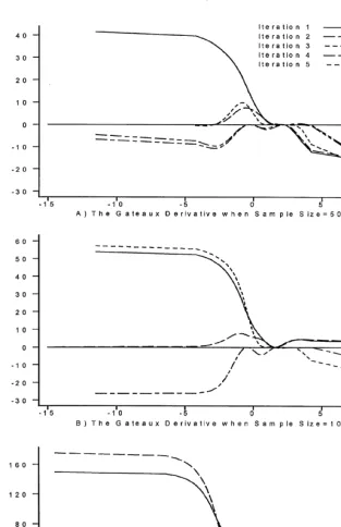
We organize the results in four steps. First we describe what happens in a single sample to both the parameters and to the Gateaux derivative as we add points of support using, respectively, Table 1 and Fig. 2. In the second subsec-tion, we look at the sampling distribution of the coe$cient on X (the source of observable heterogeneity). Here the results are summarized in Table 2. The third subsection summarizes the results for the&nuisance'parameters, that is, the"tted time function used to model duration dependence and the estimated heterogen-eity distribution. The last section looks beyond the parameter estimates and compares the true and"tted hazard functions.
5.1. A detailed look at a single sample
The example is based on a DGP that incorporates negative duration depend-ence and a discrete distribution of unobserved heterogeneity with two points of support. In the QL, the duration dependence is approximated by a cubic. In Table 1, for each iteration of the search algorithm presented in Section 2, we report: estimates of the parameter on the observable heterogeneity b; the parameters of the cubic in duration (a1}a3); and, the points of support of the distribution of unobserved heterogeneity along with their associated probabilit-ies (h
i andPi).
The results using a sample of size 500 are reported in the"rst panel. On the "rst iteration we obtain an estimate ofbwhich is far below its true value of 1.0. The cubic in duration exhibits negative duration dependence over the relevant range, but it lies everywhere above the truef(t) given by (4.3). Note that at this point we e!ectively ignore unobserved heterogeneity and observe the usual biases. The parameter on observable heterogeneity is biased towards 0, and we overestimate the degree of negative duration dependence in the hazard. More-over, the magnitude of these biases is large. The Gateaux derivative (recall that this is thenegativeof the KT multiplier of Section 2) is evaluated over a grid of candidateh's ranging from!11.51 to 11.51. The pro"le of the derivative across the grid for this iteration is reported as the solid line in panel A of Fig. 2. We see here a result which is quite common across the samples. The maximum is achieved at a corner solution: the algorithm indicates that the next point of support should be entered at the lower boundary of the grid (!11.51). This result is reported in the second last column of Table 1. Finally, in the last column of the table we report the value of the probability associated with the new point of support as calculated in Step 3 of the algorithm.
b a1 a2 a3 h1 P1 h2 P2 h3 P3 h4 P4 Log¸ hMi PMi
Sample size"500
1 0.731 2.603 !1.197 0.181 1.565 1.000 !1418.22 !11.513 0.017
2 0.740 2.224 !0.965 0.145 1.706 0.961 !25.560 0.039 !1417.39 !0.588 0.034
3 1.079 1.282 !0.626 0.098 2.788 0.528 !25.560 0.032 0.944 0.439 !1415.61 !0.847 0.067
4! 1.615 !0.879 0.347 !0.045 4.692 0.338 !0.261 0.285 2.328 0.376 !1412.57 3.106 0.004
5 1.737 !1.179 0.471 !0.062 5.115 0.285 !0.294 0.287 2.263 0.309 3.506 0.118 !1412.52
Sample size"1000
1 0.665 2.486 !1.049 0.150 1.570 1.000 !2811.36 !11.513 0.011
2 0.671 2.244 !0.900 0.125 1.658 0.975 !11.513 0.025 !2810.68 !0.987 0.036
3! 0.976 1.602 !0.752 0.113 2.785 0.464 0.980 0.536 !2808.03 !11.513 0.013
4 1.333 !0.228 0.132 !0.021 4.178 0.352 1.862 0.441 !0.442 0.207 !2804.76
Sample size"5000
1 0.670 2.558 !1.040 0.139 1.549 1.000 !14,067.84 !11.513 0.006
2 1.066 1.276 !0.563 0.077 2.935 0.493 0.852 0.507 !14,042.82 !11.513 0.008
3 1.216 0.507 !0.190 0.020 3.543 0.418 1.364 0.434 !0.292 0.147 !14,038.13 2.197 0.002
4 1.269 0.340 !0.124 0.011 3.767 0.380 0.980 0.288 !0.530 0.111 1.926 0.221 !14,037.78
Note: DGP"data generating process, QL"quasi-likelihood.bis the parameter on the observed heterogeneity, thea
iare the parameters of the cubic in duration and the
hiandP
iare the parameters of the distribution of unobserved heterogeneity. Log¸is the value of the loglikelihood.hMiis the position suggested by the search algorithm for the new point of support on the next iteration.PMiis the suggested value for the probability associated with the new point of support. DGP: Duration dependence"Negative; Unobserved heterogeneity"Discrete, Two points of support. QL: Duration dependence"Cubic.
!Indicates that a point of support was dropped in this iteration.
M.
Baker,
A.
Melino
/
Journal
of
Econometrics
96
(2000)
357
}
393
Fig. 2. The pro"le of the Gateaux Derivative. (The derivative is evaluated along the grid
11The iteration for which the QL is correctly speci"ed is number 3 for sample sizes 500 and 1000, and number 2 for sample size 5000.
suppressed its value at hK2 (!25.560) to maintain a reasonable scale in the "gure). The new maximum of the Gateaux derivative is located at!0.588. Note that in this iteration the QL is&correctly speci"ed'in the sense that it incorpor-ates a distribution of heterogeneity with two points of support. Nevertheless, the probability associated with the second point is very small and the estimate ofbis still too small.
In contrast, in the third iteration the estimate ofbis almost equal to 1.0. Also, the weight in the distribution of unobserved heterogeneity is nearly equally distributed across two points of support (h1 andh3) that are very close to the true values, while the second point continues to have small probability. Finally, the cubic exhibits less negative duration dependence than in earlier iterations. It now matches the true f(t) fairly closely up to about t"8 (about the "rst three-quarters of the sample) before diverging. Note that the Gateaux derivative displays a similar pro"le to the previous iteration and the suggested choice for the next point of support is again just less than 0.
In the fourth iteration the point of support at !25.56 is dropped, and the weight in the heterogeneity distribution is re-distributed almost equally across the remaining 3 points. This mis-speci"cation in the QL has clear e!ects on the estimates of the other parameters: the estimate ofbhas&moved beyond'1.0, and the cubic now shows signs of positive duration dependence. Similar trends are observed in the"fth and"nal iteration. The MLE ofbis more than 170% of its true value, and there is greater evidence of positive duration dependence in the a(i. This latter "nding is not surprising given the well-known result that unobserved heterogeneity can lead to spurious inference of negative duration dependence. Here, as the distribution of unobserved heterogeneity is over parameterized, the resulting &excess' negative correlation between the hazard and time is o!set by positive duration dependence in the cubic.
In the second and third panels of Table 1 and panels B and C of Fig. 2, we document the iterations in samples of 1000 and 5000 using the same DGP and QL. Very similar patterns are apparent. First, the maximum of the Gateaux derivative is often obtained at a corner solution. Second, b is estimated with reasonable precision on the iteration for which the QL is correctly speci"ed.11
Note also the rough congruence in the estimates of thea
iacross samples on this iteration. Third, the NPMLE leads to an over-parameterization of the distribu-tion of unobserved heterogeneity. Fourth, the MLE of the cubic displays relative positive duration dependence to o!set this mis-speci"cation.
A summary of estimates ofbacross DGPs and quasi likelihoods
DD: none DD: none 1.000 1.007! 1.004 1.000 0.992 0.993! 0.996 0.993 0.998 0.998! 0.999 0.998
Het.: none (0.108) (0.108) (0.110) (0.108) (0.068) (0.071) (0.069) (0.068) (0.033) (0.033) (0.033) (0.033)
DD: cubic 1.001 1.123! 1.394 1.011 0.992 1.079! 1.177 1.001 0.997 1.033! 1.075 0.997
(0.117) (0.181) (0.505) (0.140) (0.076) (0.117) (0.219) (0.106) (0.036) (0.053) (0.076) (0.036)
DD: step 1.004 1.149 4.023 1.012 0.993 1.079 3.289 0.996 0.997 1.039 2.499 0.997
(0.118) (0.181) (1.813) (0.132) (0.076) (0.125) (1.295) (0.084) (0.036) (0.055) (0.879) (0.036)
DD: none DD: none 0.905 1.015 1.028 1.015 0.896 1.004 1.012 1.004 0.901 1.005 1.010 1.006
Het.: discrete (0.118) (0.132) (0.132) (0.132) (0.083) (0.091) (0.091) (0.091) (0.039) (0.042) (0.043) (0.042)
DD: cubic 0.701 0.959! 1.372 0.827 0.692 0.967! 1.148 0.875 0.698 0.990 1.062 1.011
(0.086) (0.226) (0.594) (0.234) (0.060) (0.173) (0.225) (0.228) (0.029) (0.077) (0.065) (0.053)
DD: step 0.702 1.003 3.436 0.843 0.697 0.995 2.914 0.901 0.698 0.998 2.268 1.010
(0.087) (0.206) (1.559) (0.247) (0.060) (0.161) (0.875) (0.238) (0.029) (0.068) (0.845) (0.051)
DD: none DD: none 0.776 0.981 1.003 0.984 0.774 0.981 0.998 0.983 0.766 0.980 0.998 0.993
Het.: Gamma (0.150) (0.132) (0.133) (0.132) (0.115) (0.099) (0.100) (0.098) (0.051) (0.043) (0.044) (0.045)
DD: cubic 0.651 0.943 1.430 0.944 0.649 0.942 1.164 0.952 0.642 0.940 1.060 0.960
(0.113) (0.158) (0.644) (0.198) (0.087) (0.111) (0.225) (0.128) (0.036) (0.046) (0.084) (0.066)
DD: step 0.652 0.948 3.917 0.946 0.650) 0.943 3.491 0.954 0.643 0.940 2.631 0.966
(0.113) (0.154) (1.461) (0.181) (0.087) (0.111) (1.310) (0.119) (0.036) (0.046) (0.896) (0.073)
DD: negative DD: none 1.191 1.260 1.310 1.265 1.198 1.273 1.316 1.284 1.194 1.261 1.303 1.290
Het.: none (0.120) (0.135) (0.142) (0.137) (0.081) (0.096) (0.099) (0.101) (0.040) (0.044) (0.047) (0.051)
DD: cubic 1.011 1.140! 1.523 1.042 1.014 1.126! 1.339 1.045 1.005 1.057 1.200 1.030
(0.101) (0.155) (0.483) (0.209) (0.067) (0.132) (0.241) (0.123) (0.035) (0.057) (0.094) (0.080)
DD: step 1.012 1.160 4.212 1.027 1.015 1.144 3.913 1.026 1.004 1.049 2.608 1.004
(0.102) (0.152) (1.473) (0.131) (0.068) (0.134) (1.203) (0.087) (0.034) (0.050) (1.031) (0.034)
DD: negative DD: none 0.897 1.138 1.325 1.223 0.890 1.128 1.310 1.250 0.867 1.107 1.269 1.249
Het.: discrete (0.152) (0.232) (0.240) (0.269) (0.105) (0.162) (0.175) (0.181) (0.048) (0.070) (0.077) (0.077)
DD: cubic 0.678 0.897! 1.409 0.830 0.676 0.929 1.247 0.885 0.662 0.901 1.152 1.054
(0.110) (0.246) (0.523) (0.337) (0.077) (0.184) (0.264) (0.283) (0.036) (0.163) (0.109) (0.108)
DD: step 0.677 0.995 4.123 0.813 0.674 0.980 3.670 0.829 0.660 0.987 2.768 0.994
(0.110) (0.223) (1.744) (0.340) (0.077) (0.162) (1.247) (0.264) (0.036) (0.084) (0.823) (0.076)
DD: cubic 0.721 1.001 1.411 0.958 0.727 0.995 1.258 1.011 0.723 0.977 1.166 1.028 (0.114) (0.151) (0.386) (0.234) (0.087) (0.128) (0.230) (0.174) (0.038) (0.051) (0.099) (0.104)
DD: step 0.721 1.004 4.253 0.951 0.727 0.997 3.992 0.983 0.722 0.973 2.898 0.975
(0.115) (0.150) (1.817) (0.222) (0.087) (0.120) (1.174) (0.154) (0.038) (0.051) (1.155) (0.053)
DD: positive DD: none 0.803 0.803 0.803 0.795 0.795 0.795 0.795 0.795 0.795
Het.: none (0.074) (0.074) (0.074) (0.055) (0.055) (0.055) (0.026) (0.026) (0.026)
DD: cubic 1.008 1.147! 1.954 1.024 0.995 1.099! 1.407 1.003 0.994 1.048! 1.061 0.994
(0.101) (0.156) (1.183) (0.154) (0.076) (0.121) (0.783) (0.096) (0.036) (0.059) (0.086) (0.036)
DD: step 1.012 1.172 4.003 1.039 0.998 1.118 3.529 1.009 0.994 1.048 2.851 0.994
(0.103) (0.162) (1.981) (0.177) (0.076) (0.131) (1.541) (0.102) (0.036) (0.063) (1.258) (0.036)
DD:positive DD: none 0.796 0.806 0.808 0.806 0.795 0.807 0.808 0.808 0.794 0.806 0.807 0.806
Het.: discrete (0.110) (0.113) (0.113) (0.113) (0.075) (0.077) (0.077) (0.077) (0.031) (0.032) (0.032) (0.032)
DD: cubic 0.712 0.946! 1.299 0.800 0.711 0.953! 1.104 0.863 0.707 0.969! 1.008 0.978
(0.098) (0.205) (0.659) (0.214) (0.067) (0.171) (0.256) (0.208) (0.029) (0.097) (0.092) (0.088)
DD: step 0.715 0.974 2.910 0.835 0.712 0.958 2.607 0.893 0.708 0.966 2.317 0.988
(0.098) (0.205) (1.297) (0.259) (0.067) (0.165) (0.816) (0.245) (0.029) (0.097) (0.855) (0.067)
DD: positive DD: none 0.667 0.794 0.800 0.794 0.670 0.796 0.801 0.796 0.664 0.789 0.792 0.789
Het.: Gamma (0.132) (0.105) (0.107) (0.105) (0.103) (0.076) (0.077) (0.076) (0.043) (0.033) (0.034) (0.033)
DD: cubic 0.627 0.908 1.413 0.935 0.629 0.920 1.188 0.959 0.623 0.919 1.042 0.991
(0.101) (0.146) (0.562) (0.173) (0.077) (0.130) (0.263) (0.123) (0.031) (0.040) (0.070) (0.056)
DD: step 0.632 0.916 3.709 0.952 0.632 0.911 3.200 0.937 0.625 0.909 2.555 0.972
(0.102) (0.136) (1.550) (0.240) (0.077) (0.102) (1.025) (0.125) (0.031) (0.040) (0.927) (0.074)
Note: DGP"data generating process. DD"duration dependence; Het."unobserved heterogeneity. The reported statistics are the mean and standard deviation of across 100 samples on the indicated iteration of the algorithm. Initial"on the"rst iteration; Two points"on the iteration in which the distribution of unobserved heterogeneity is speci"ed as
having two points of support; MLE"the maximum likelihood estimate; HQIC"the estimate using the Hannon Quinn Information Criterion. An empty cell indicates that the algorithm always stopped with the"rst point of support.
!Means calculated over less than 100 samples, as the search algorithm stopped before reaching the the second point of support.
12Our calculations were done on a Pentium 133 PC. We used a Watcom Fortran compiler. For Step 1, we reparameterized the probabilities via a logistic transformation to constrain them to the unit simplex. We then used repeated calls to the DFP algorithm from GQOPT to guarantee convergence. The calculations in Table 2 took about 5 months of CPU time.
13Sin and White (1996) survey the properties of various information measures in a wide variety of settings.
14Using the BIC in place of the HQIC sometimes leads to the selection of models with fewer points of support, but the statistics reported in Table 2 would be virtually identical if we used the BIC rather than the HQIC.
parameters of the model. This tendency is not attenuated to any large degree as sample size grows over the range typically encountered in longitudinal data sets. In the next section we provide evidence that this conclusion remains true across a wide variety of DGPs and QLs.
5.2. Sampling distribution ofb
In Table 2 we report the mean and standard deviation for the estimates ofbin the 81 experimental settings.12 For each of our nine DGPs, we took the 100 simulated samples and estimatedbusing each of the three QLs and the three sample sizes. To show how the estimates vary as we add points of support to the distribution of the unobserved heterogeneity, we report the statistics at 4 values forNK h:NK h"1;NK h"2;NK h"NK MLEh andNK h"NK HQh (de"ned below).
The results when NK h"1 allows us to judge the consequences of ignoring unobserved heterogeneity whether or not that is the right thing to do. Many researchers"x the valueN
hto 2, a priori. The results whenNK h"2 demonstrate
the performance of this ¶metric'speci"cation. The third column contains the descriptive statistics for the estimatedbwhenNK his chosen according to the nonparametric MLE described in Section 2. Our fourth column is based on estimatingNK h by the Hannan-Quinn Information Criterion (HQIC). Informa-tion criterion are typically of the form
ln¸!cp (5.1)
wherepis the number of parameters in the model andcis a penalty function. The Schwarz or Bayesian Information Criterion (BIC) sets c"ln (N
h)/2. The HQIC sets c"ln (ln (N
The results in Table 2 lead to the following conclusions about the estimates ofb:
First, a nonparametric speci"cation for either duration dependence or unob-served heterogeneity, when the other feature is known to be absent, leads to estimates that are well behaved for all sample sizes considered.
Second, mis-speci"cation matters. Although it is di$cult to distinguish unob-served heterogeneity from duration dependence, it is not su$cient to model one of these features in a#exible way while ignoring the other as suggested by some authors (e.g. Meyer, 1990; Ridder, 1987). This practice can lead to signi"cant biases.
Third, the combination of a#exible speci"cation for both duration depend-ence and the distribution of unobserved heterogeneity leads to a large and systematic bias for the estimatedbthat declines very slowly with sample size. It appears that the poor sampling performance stems almost entirely from the fact that the NPMLE"nds too many&spurious'points of support and overestimates the dispersion of the unobserved heterogeneity while compensating for this mis-speci"cation through the estimate of the duration dependence. The excess-ive dispersion causes the hazard to decline too sharply with time. A #exible speci"cation for /(t) in the QL allows the NPMLE to o!set the e!ects of excessive dispersion of the unobserved heterogeneity on the hazard with spuri-ous positive duration dependence. Notice that this interaction and the resulting problems do not arise when there is no duration dependence in either the DGP or the QL. Excessive dispersion of the unobserved heterogeneity also leads to a large bias in the estimated b. It is well known that ignoring heterogeneity biases the estimate ofb towards zero. We"nd that the NPMLE leads to an estimatedbthat is biased away from zero. Moreover, this bias is so large that, for the sample sizes considered, researchers would be better o! ignoring the unobserved heterogeneity altogether.
Our fourth "nding is that the problems associated with the NPMLE are greatest when the true DGP displays negative duration dependence. Unfortu-nately, this is probably the case of greatest interest to applied researchers.
many cases, we do almost as well in large samples as we could if we actually knew the true value ofN
h. However, for sample sizes of 500 or 1000, we see (at
least with some DGPs) that the penalized MLE displays a slight negative bias when the QL has either a cubic or a step function. The HQIC in these situations is conservative in that better parameter estimates would have been obtained if the penalty on adding points of support was reduced.
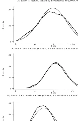
In Fig. 3, we plot a kernel density estimate of the sampling distribution for
bK obtained using the HQIC, for a few cases. We also plot a normal density standardized to have the same mean and variance. To conserve space, we restrict attention to the case where the DGP has no duration dependence, the QL has a cubic polynomial and the sample size is 5000. Because we only have 100 draws for each experiment, these graphs provide at best a rough guide to the unknown large sample distribution of the estimatedb. Nonetheless, it appears that in these three cases, a normal approximation to the sampling distribution seems to work reasonably well. Unfortunately, in other cases we"nd that a normal approxima-tion is much less reliable. In smaller samples, thebK obtained using the HQIC often has bimodal distribution. The second mode appears to decline with sample size, but in several of our designs, the second mode is still noticeable even with a sample size of 5000. The corresponding plots for the NPMLE estimator of
b (not shown) reveal that although it is very badly biased in many cases, the sampling distribution appears to be fairly well approximated by a normal density in large samples for all the DGP/QL pairs in our design.
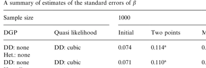
Although there is no asymptotic theory to justify it, practitioners routinely compute and report standard errors for the NPMLE based on inverting the Hessian. Table 3 gives the average standard errors for bK so obtained at
NK h"1,NK h"2,NK h"NK MLEh , andNK h"NK HQh for the same DGPs and QL used to construct Fig. 3, but using a smaller sample size of 1000. Comparing to Table 2, we see that these standard errors tend to underestimate the sampling standard deviations and these biases are particularly large for both the NPMLE and the penalized MLE.
5.3. Sampling distribution of estimated duration dependence and heterogeneity distribution
Table 3
A summary of estimates of the standard errors ofb
Sample size 1000
DGP Quasi likelihood Initial Two points MLE HQIC
DD: none DD: cubic 0.074 0.114! 0.172 0.074
Het.: none
DD: none DD: cubic 0.071 0.110! 0.189 0.091
Het.: discrete
DD: none DD: cubic 0.070 0.094 0.180 0.095
Het.: Gamma
Note: DGP"data generating process. DD"duration dependence; Het."unobserved heterogen-eity. The reported statistics are the mean of the estimated standard errors ofbacross 1000 samples on the indicated iteration of the algorithm. Initial"on the"rst iteration; Two points"on the iteration in which the distribution of unobserved heterogeneity is speci"ed as having two points of support; MLE"the maximum likelihood estimate; HQIC"the estimate using the Hannon-Quinn Information Criterion.
!Means are calculated over less than 100 samples, as the search algorithm stopped before reaching the the second point of support.
the estimated duration dependence function are closely related. Estimates of
b below 1 are usually accompanied by excessively negative duration depend-ence. Conversely, estimates ofb above 1 are usually accompanied by positive bias in the estimated duration dependence.
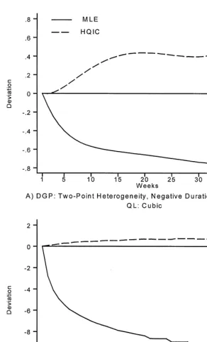
For example, in panel A if Fig. 4 the true DGP displays negative duration dependence and a two-point heterogeneity distribution, and the QL has a cubic time polynomial. The average estimated value of/(t) obtained with the penaliz-ed MLE overestimatesf(t). Note from Table 2 that the average value ofbin this case is 0.885. In contrast, using the NPMLE leads to an estimated value of/(t) that is on average below the true value. Recall that in our parameterization, negative values of/(t) correspond to a hazard that isincreasingwith duration, so the NPMLE is biased toward positive duration dependence. This bias in the time function matches up with a bias inb; the average estimated value here is 1.247 (Table 2).
dependence. Although ignoring the unobserved heterogeneity or trying to capture it with a tightly parameterized heterogeneity distribution leads to estimates of negative duration dependence, they "nd that the NPMLE indicates positive duration dependence in these data. Our results suggest that this reversal in the estimated duration dependence may be due to the small sample bias associated with the NPMLE rather than the relaxation of an incorrect speci"cation. More generally, our results suggest that"nding positive duration dependence is even more likely if we combine the NPMLE with a#exible speci"cation of the baseline hazard.
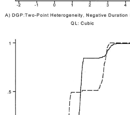
The distribution of unobserved heterogeneity is usually treated as a nuisance parameter and is rarely of direct interest. In part, this re#ects the belief that this distribution cannot be estimated with much precision. We"nd that the NPMLE is in fact a poor estimator. It often leads to an estimated distribution that is incorrectly centred and tends to put to much probability on extreme values forh. In contrast, use of the HQIC leads to a much more reliable estimator. In Fig. 5, we plot the average estimated distribution function of unobserved heterogeneity obtained via the HQIC for the two cases described above. The agreement between the true and average"tted cumulative distribution function is remarkably good, and it clearly improves with sample size.
5.4. Predicted hazards
Although the separate components of the hazard are di$cult to estimate and can be subject to large biases, particularly if we overparameterize, maximizing the QL virtually guarantees a close"t between the observed and the predicted hazards. Let jt(X) denote the exit hazard at time t for an individual with observable characteristicsX. The predicted hazard is constructed as a weighted sum of the hazardsjit(X) for an individual of typei. The weightsw
it~1(X) give
the probability that an individual with observable characteristicsX who has survived to timet!1 is of typei. With discrete types, we have
j
t(X)"+ i
j
it(X)wit~1(X).
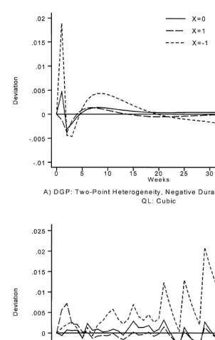
In Fig. 6, we plot the di!erence between the true hazard and the average of the predicted hazards for three values ofX (the observed heterogeneity). The predicted hazards are formed using the NPMLE estimates. The three values of
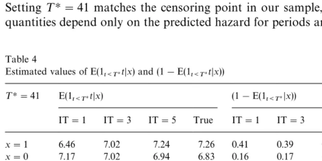
Table 4 Note: Estimates are obtained using the parameter values from the "rst panel of Table 1 (500 observations). IT"iteration. The statistics in the columns labelled&True'are constructed using the true parameter estimates.
X is unlikely to survive in the sample for very long (e.g., X"!1). In such a case, the observed hazard at long durations is uninformative and cannot impose agreement between the true and predicted hazards.
Many questions of interest to researchers depend on the structural para-meters only through the predicted hazard. Notable examples are the expected duration of a spell given the vector of observablesX
1, or the expected change in
duration if the observables are varied fromX
1toX2. For such questions, the
di$culty in estimating the structural parameters is largely irrelevant if the values ofX
1andX2are&well-represented'in the sample, and we can ignore censoring.
In practice, the predicted hazard often leads to a defective distribution for duration (that is, it gives a nonzero probability to the event that the spell never ends), so the expected duration is not well de"ned. Let 1
t:TH denote the
indicator variable that equals 1 if the duration t is less than ¹H, and zero otherwise. It is convenient to summarize the"tted hazard via the estimates for the two quantities E(1
t:THtDX) and (1!E(1t:THDX)) at various values for¹H. As
¹Hincreases toR, E(1
t:THtDX) converges to E(tDX) when the latter exists, but it
is also well behaved for most defective distributions. (1!E(1
t:THDX)) gives the
probability that a spell does not end before time¹H.
Using the parameter estimates from the"rst panel of Table 1 (that is, those obtained with 500 observations), we computed E(1
t:THtDX) and
(1!E(1
t:THDX)), at various values of X. The results are reported in Table 4.
15Using data from the Slovak Republic, Ham et al. (1998) estimate the impact of an additional week's entitlement to unemployment insurance on the expected duration of an unemployment spell. They report that the predicted duration rises from 0.4 to 1.1 to 1.9 weeks as the number of points of support in the"tted heterogeneity distribution increases from 1 to 2 to 3, respectively.
are observed. Although the parameter values change dramatically as we go from iteration 1 to 5 (among other things, the coe$cient on observed heterogeneity increases from 0.73 to 1.74), the values for the two summaries of the predicted hazard duration barely change. Researchers may also be interested, however, in using the structural parameters to explore out of sample experiments. For example, a researcher may want to know the impact of a change inX on the expected duration for complete spells. With censoring, the sample data are only partially informative and the predicted hazard must be extrapolated beyond the observed range of the data. As a consequence, bias in the estimated structural parameters can have important consequences. Ham et al. (1998) report that the predicted expected duration for complete spells can be very sensitive to the number of points in the estimated heterogeneity distribution.15 Although we "nd that extrapolating the cubic polynomial beyond the range of the data never works well, we obtain a similiar sensitivity to the number of points of support using our example in Table 4. In our case, the predicted distribution for duration is defective at 1 point support (so the mean duration is in"nite), but duration has a"nite mean when we use the estimates from the NPMLE.
6. Some extensions
This section contains some extensions that we have investigated but not as intensively as in the main Monte Carlo.
6.1. Very large samples
The results reported in Table 2 show that estimates ofbdisplay large biases when we combine the NPMLE of the heterogeneity distribution with a#exible duration dependence speci"cation in the QL. However, the bias appears to decline with sample size. In order to investigate more fully the e!ect of sample size, we combined our 100 samples of 5000 observations into 5 samples each containing 100,000 observations. To reduce computational costs, we considered only the cases where the true DGP displays no duration dependence. Note that this implies that all the QL speci"cations contain the true DGP as a special case. The results of the nine experiments are reported in Table 5.
Table 5
A summary of estimates ofbin large samples
Sample size 100 ,000
DGP Quasi likelihood Initial Two points MLE HQIC
DD: none DD: none 0.997 0.997! 0.998 0.997
Het.: none (0.008) (0.009) (0.008) (0.008)
DD: cubic 0.996 0.999 1.008 0.996
(0.009) (0.010) (0.012) (0.009)
DD: step 0.996 0.999 1.079 0.996
(0.009) (0.010) (0.098) (0.009)
DD: none DD: none 0.901 1.005 1.006 1.005
Het.: discrete (0.008) (0.008) (0.008) (0.008)
DD: cubic 0.698 1.004 1.011 1.004
(0.007) (0.010) (0.011) (0.010)
DD: step 0.697 1.005 1.128 1.005
(0.007) (0.010) (0.110) (0.010)
DD: none DD: none 0.765 0.979 0.996 0.996
Het.: Gamma (0.016) (0.010) (0.009) (0.009)
DD: cubic 0.642 0.938 1.000 0.989
(0.012) (0.010) (0.013) (0.012)
DD: step 0.642 0.938 1.169 0.989
(0.012) (0.010) (0.150) (0.012)
Note: DGP"data generating process. DD"duration dependence; Het."unobserved heterogen-eity. The reported statistics are the mean and standard deviation ofbacross 5 samples on the indicated iteration of the algorithm. Initial"on the"rst iteration; Two points"on the iteration in which the distribution of unobserved heterogeneity is speci"ed as having two points of support; MLE"the maximum likelihood estimate; HQIC"the estimate using the Hannon-Quinn In-formation Criterion.
!Means are calculated over less than 5 samples, as the search algorithm stopped before reaching the second point of support.
by imposing a priori the true number of points of support. The biases are negligible and the standard errors decline roughly in line with the square-root of sample size. When the unobserved heterogeneity is drawn from a gamma distribution, use of the HQIC leads to estimates that are very close to the true value. If anything, however, the estimator is a bit conservative when the QL contains either a cubic or step function in that better estimates would have been obtained if the penalty on the number of parameters was slightly smaller.
6.2. Increasing thevariance of observable heterogeneity
An increase in the variance of observed heterogeneity should reduce the sampling variance ofbK and may help to distinguish the relative contributions of duration dependence and unobserved heterogeneity. To investigate the con-sequences of increasing p2
x, we conducted the following experiment. It was not feasible to consider all nine combinations of duration dependence and unobserved heterogeneity, so we restricted attention to a DGP with negative duration dependence and a discrete heterogeneity distribution with two points of support. We increased the variance ofX, p2
x, from 0.25 to 1.00. To maintain comparability with the results from Section 5, we used exactly the same draws from the heterogeneity distribution and the values of X were simply multiplied by two. Once again, we used the speci"ed DGP to generate 100 samples of 5000 observations. The increase inp2xhad some minor e!ects on the distribution of observed duration: the average duration of a spell increased by about 0.6 to 14.86, and the fraction of censored observations increased margin-ally from about 19% to 21%. However, the increase inp2
xdid have a large e!ect on the relative importance of observed heterogeneity: the average R2 from a regression of log-duration onXacross the 100 samples jumped from 0.071 to 0.228.
Table 6 summarizes the results. We see that the increase in p2
x results in a marginal improvement in the sampling distribution of the MLE and penalized MLE but does not alter the substantive conclusions reached in Section 5.
6.3. A computational alternative
Using the value ofhthat maximizes the Gateaux derivative in Step 2b of our algorithm, as suggested by Heckman and Singer, often leads to a corner solution; i.e., the value ofhso chosen is either extremely large or extremely small. This choice has potentially important consequences for both computational e$ciency and inference. For example, an extreme point of support may be added on the second or third iteration of our algorithm only to spend many CPU cycles bringing it back to something in the&middle'of our chosen range. In other cases, the algorithm"nds a local optimum at an extreme value ofhbut assigns it a negligible probability, so that the quasilikelihood barely increases. Because the HQ criterion is sensitive to the order in which points of support are added, adding a point with negligible probability on the second iteration of our algorithm can lead the HQ criterion to settle for too little heterogeneity. Both of these issues are nicely illustrated by our example in Section 5.1.
Table 6
Estimates ofbwhen the variance of observable heterogeneity is increased
Sample size 500 1000 5000
DGP Quasi likelihood
Initial Two points
MLE HQIC Initial Two points
MLE HQIC Initial Two points
MLE HQIC
DD: negative DD: none 0.906 1.205 1.294 1.246 0.902 1.190 1.282 1.255 0.914 1.192 1.281 1.267 Het.: discrete (0.071) (0.098) (0.109) (0.110) (0.054) (0.071) (0.073) (0.077) (0.027) (0.037) (0.037) (0.038)
DD: cubic 0.687 0.962 1.302 0.977 0.683 0.960 1.204 1.013 0.690 0.984 1.122 1.033 (0.055) (0.170) (0.284) (0.223) (0.039) (0.147) (0.146) (0.137) (0.019) (0.109) (0.068) (0.057) DD: step 0.685 0.994 3.551 0.919 0.681 0.984 3.295 0.972 0.687 0.996 2.130 1.001
(0.056) (0.146) (1.376) (0.212) (0.039) (0.108) (1.341) (0.178) (0.019) (0.059) (1.015) (0.050)
Note: DGP"data generating process. DD"duration dependence; Het."unobserved heterogeneity. The reported statistics are the mean and standard deviation ofbacross 100 samples on the indicated iteration of the algorithm. Initial"on the"rst iteration; Two points"on the iteration in which the distribution of unobserved heterogeneity is speci"ed as having two points of support; MLE"the maximum likelihood estimate; HQIC"the estimate using the Hannon-Quinn Information Criterion. For these results, the variance of observable heterogeneity (X) is set to 1.00 (it is set to 0.25 for the results in Tables 1}3).
Baker,
A.
Melino
/
Journal
of
Econometrics
96
(2000)
357
}
393
16The only di!erence is that in these examples our suggestion for choosing the new candidate never lead us to add a point of support on one interation only to drop it on the next.
maximize a quadratic approximation. More precisely, we can re-write slightly the problem faced in (2.3) as
max
on havingNM hpoints of support, and wherehM is the candidate for the next point of support. Suppose we choose q to maximize a second order Taylor series approximation to the right-hand side of (6.1). Then, in Step 2b of our algorithm, we choose the candidatehM that yields the highest value for
+
Notice that the numerator in (6.2) is the Gateaux derivative. The same terms appear in both numerator and denominator of (6.2), so choosing the new point of support is only marginally more di$cult than in the original Heckman and Singer (1984) approach. Also, this alternative rule shares the desirable property that the selected value ofhis guaranteed to increase the likelihood function.
We found that our second-order method for choosingh was less likely to wander o!to a corner. For instance, in the three samples reported in Table 1, maximizing the Gateaux derivative lead us four times to a corner value of
!11.513. In contrast, maximizing (6.2) only lead us to the corner once. Al-though it saved some CPU cycles, maximizing (6.2) did not a!ect the parameter estimates. We reached exactly the same MLE conditional on the number of points of support as reported in Table 1.16
additional points of support lead to identical NPMLE estimates ofbin all cases, and to the same estimates conditional on a given number of points of support in the vast majority of cases. In the few cases where di!erent local optima where reached conditional on the number of points of support, neither rule lead to consistently higher values for the quasilikelihood.
7. Conclusion
Our Monte Carlo results demonstrate that recent improvements in com-puting power, coupled with some care in designing the algorithm, make it computationally feasible to combine the NPMLE estimator of the unobserved heterogeneity distribution with a very#exible speci"cation for duration depend-ence. However, our results also show that this estimation strategy has poor sampling properties.
We"nd that a nonparametric speci"cation for either duration dependence or unobserved heterogeneity, when the other feature of the hazard is known to be absent, leads to estimators that are well behaved even in modestly sized samples. However, the combination of a#exible speci"cation for both duration depend-ence and unobserved heterogeneity leads to very reliable and systematic biases in each of the components of the estimated hazard. Applied researchers often sacri"ce e$ciency by adding extra parameters to safeguard against mis-speci-"cation. Our results suggest that this strategy is particularly questionable in this setting. Adding super#uous parameters not only sacri"ces e$ciency, it also introduces a potentially very large bias, even in very large samples. With a #exible speci"cation for duration dependence, the NPMLE is biased towards "nding an excessively dispersed distribution of unobserved heterogeneity. The "t to the empirical hazard is maintained by compensating with a positive bias to the estimated duration dependence and a bias to the coe$cient on observed heterogeneity away from zero. In fact, we found (almost without fail) that the estimates of/(t) andbmoved in the directions consistent with these biaseseach
time we added a point of support to our estimated heterogeneity distribution. On the other hand, ignoring unobserved heterogeneity leads to a negative bias in estimated duration dependence and biases the coe$cient on observed hetero-geneity towards zero.
Acknowledgements
We gratefully acknowledge the research support of SSHRC. We thank David Green, John Ham, Jim Heckman, Tom Mroz and Gary Solon for helpful comments. Mike Campolieti provided invaluable research assistance.
References
Baker, M., Rea, S., 1998. Employment spells and unemployment insurance eligibility requirements. Review of Economics and Statistics 80, 80}94.
Cameron, S.V., Heckman, J.J., 1998. Life cycle schooling and dynamic selection bias: models and evidence for"ve cohorts of American Males. Journal of Political Economy 106, 262}333. Campolieti, M., 1997. Bayesian estimation of discrete duration models. Ph.D. Thesis, University of
Toronto.
Cosslett, R., 1983. Distribution-free maximum likelihood estimator of the binary choice model. Econometrica 51, 765}782.
Elbers, C., Ridder, G., 1982. True and spurious duration dependence: the identi"ability of the proportional hazards model. Review of Economic Studies 49, 402}411.
Hahn, J., 1994. The e$ciency bound of the mixed proportional hazard model. Review of Economic Studies 61, 607}629.
Ham, J.C., Rea Jr., S.A., 1987. Unemployment insurance and male unemployment in Canada. Journal of Labor Economics 5, 325}353.
Ham, J.C., Svejnar, J., Terrell, K., 1998. Unemployment, the social safety net and e$ciency in transition: evidence from micro data on Czech and Slovak men. American Economic Review 88, 1117}1142.
Heckman, J., Singer, B., 1984. A method for minimizing the impact of distributional assumptions in econometric models for duration data. Econometrica 52, 271}320.
Huh, K., Sickles, R.C., 1994. Estimation of the duration model by non-parametric maximum likelihood, maximum penalized likelihood, and probability simulators. The Review of Econ-omics and Statistics 76, 683}694.
Ishwaran, H., 1996. Uniform rates of estimation in the semiparametric Weibull mixture model. The Annals of Statistics 24, 1572}1585.
Lancaster, T., 1979. Econometric methods for the duration of unemployment. Econometrica 47, 939}956.
Lancaster, T., 1990. The Econometric Analysis of Transition Data. Cambridge University Press, Cambridge.
Lemieux, T., MacLeod, W.B., 1995. State dependence and unemployment insurance. Human Resources and Development Canada, Ottawa.
Leroux, B.G., 1992. Consistent estimation of a mixing distribution. The Annals of Statistics 20, 1350}1360.
Lindsay, B.G., 1983. The geometry of mixture likelihoods: a general theory. The Annals of Statistics 11, 86}94.
Lindsay, B.G., Lesperance, M.L., 1995. A review of semiparametric mixture models. Journal of Statistical Planning and Inference 47, 29}39.
Luenberger, D.G., 1984. Linear and Nonlinear Programming, 2nd Edition. Addison-Wesley, Read-ing, MA.
Meyer, B.D., 1990. Unemployment insurance and unemployment spells. Econometrica 58, 757}782. Narendranathan, W., Stewart, M.B., 1993. How does the bene"t e!ect vary as unemployment spells
Nickell, S., 1979. Estimating the probability of leaving unemployment. Econometrica 47, 1249}1266. Ridder, G., 1987. The sensitivity of duration models to misspeci"ed unobserved heterogeneity and
duration dependence. Working Paper, University of Groningen.
Ridder, G., 1990. The non-parametric identi"cation of generalized accelerated failure-time models. Review of Economic Studies 57, 167}182.
Sider, H., 1985. Unemployment duration and incidence: 1968}82. American Economic Review 75, 461}472.
Sin, C.-Y., White, H., 1996. Information criteria for selecting possibly misspeci"ed parametric models. Journal of Econometrics 71, 207}225.