Some rules of Probability and Statistics

(1)

MA8017 Engineering Mathematics Halmstad University

Some rules of Probability and Statistics

Def If an experiment hasm outcomes of whichb results in the event A, then the probability of A is

P(A) = g/m .

Def P is a probability measure if 1. 0≤P(A)≤1

2. P(Ω) = 1

3. A_∩B =_{∅ ⇒} P(A_∪B) = P(A) +P(B) for all eventsA ⊂Ω where Ω is the sample space.

Basic principle If an experiment can be divided into j subexperiments where the of counting first hasn1 outcomes

second has n2 outcomes ...

jth has nj outcomes

then the experiment totally has n1·n2· · ·nj outcomes.

Addition theorem P(A_∪B) = P(A) +P(B)₋P(A_∩B).

Def A and B are independent events if P(A∩B) = P(A)P(B)

Def The conditional probability ofA givenB is P(A_|B) = P(A∩B)

P(B)

Bayes theorem If A1, . . . , An is a partition of Ω (i.e. i6=j ⇒Ai∩Aj =∅ and Sn

i=1Ai = Ω).

then P(Ak_|B) = PnP(B|Ak)P(Ak)

i=1P(B|Ai)P(Ai)

for each k = 1,2, . . . , n.

Combinatorics The number of ways to choosek elements amongn possible, without replacement and without respect to the order, is

n k

= n!

k! (n−k)! =

n(n₋1)_{· · ·}(n₋k+ 1)

(2)

Random X discrete: Probability fcn: p(x) = P(X =x)

variables Distribution fcn: P(X ≤a) = F(a) = P

x≤ap(x),

X cont.: Density fcn: f(x) = _dxdP(X ≤x) Distribution fcn: P(X _≤a) = F(a) = Ra

−∞f(x)dx.

Expected value X discrete: The expected value of X: µ=E(X) = P

x∈Ωx p(x).

and variance Variance of X: σ2 ₌_V₍_X_{) =} P

x∈Ω(x−µ)2p(x).

X cont: Expected value of X: µ=E(X) = R

x∈Ωx f(x)dx. Variance of X: σ2 ₌_V₍_X_{) =} R

x∈Ω(x−µ)

2_f₍_x₎_dx_.

Covariance of X and Y: C(X, Y) = E((X₋µx)(Y ₋µy)) Correlation of X and Y: ρ = √C(X,Y)

V(X)V(Y) Standarddev. σ = p

V(X).

Linearity: E(aX+bY) = a E(X) +b E(Y) for all random variables X and Y and real numbers a and b.

IfX, Y indep. then V(aX+bY) = a2_V₍_X_{) +}_b2_V₍_Y_). Rules: E(g(X)) = R

Rg(x)f(x)dx

V(X) = E(X2₎₋₍_E₍_X₎₎2

C(X, Y) = R R

R2xy f(x, y)−E(X)E(Y) C(P

iaiXi,

P

kbkYk) =

P

i

P

kaibkC(Xi, Yk)

Normal denoted by N(µ, σ2_{) where}_µ _{is the expected value and}_σ2 _{is the variance} distributionN(0,1) is called standard normal distribution with density function Φ(x)

If X _∈N(µ, σ2_{) then}_P₍_X _≤_x_{) = Φ} x−µ σ

Symmetry: Φ(−x) = 1−Φ(x)

Probabilities: P(a _≤X _≤b) = Φ b−_σµ

−Φ a−_σµ

Def The random variables X1, X2, . . . , Xn are a sample ofX if all variables, Xi, is distributed asX, i= 1, . . . , n, and all variables are independent of

each other at all levels.

CLT (Central Limit Theorem)

If X1, . . . , Xn is a sample where

E(Xi) =µ and V(Xi) = σ2,i= 1, . . . , n

then P√_σn( ¯X−µ)≤x → Φ(x) as n→ ∞. This implies that Pn

i=1Xi is approximately N(nµ, nσ2)

and ¯X is approximately N(µ, σ2_/n_{) for large}_n_.

Approximations Distribution Condition Approximative distribution

Bin(n, π) n _≥10 andπ <0.1 P o(nπ)

Bin(n, p) np(1₋p)_≥10 N(np, np(1₋p))

(3)

Def _{Xt_}=_{Xt:t _∈T _⊆R} is a random process if all variables Xt, t_∈T have the same probability distribution regardless of t. T is called index space.

Thm If _{Xt_} has independent, stationary increments and X0 = 0 then rX(s, t) = min(s, t)·V(X1).

Relationship between cvf, r(τ), and spectral density,R(f),

Continuous time Discrete time

If {Xt} is a random process which is sampled into {Yk}={Xkd :k = 0,±1,±2, . . .} (normed frequency)

If _{Xt} is the shot-noise process with parameter λ and pulse-function g(s)

(4)

Relation to cvf

Relation between spectral density and transfer function

RY(f) =_|H(f)_|2_RX₍_f₎

Def White noise in discrete time is an independent sequence _{ǫt_}∞

(5)

Def The cross covariance of _{Xt_} and _{Yt_} is denoted by rX,Y(τ) and defined by rX,Y(τ) = C(Xt, Yt+τ) =

R Re

i2πf τ_RX,Y₍_f₎_df

Derivative process

Thm Ifr_X′′(τ) exists then {Xt′} exists and then

rX′(τ) = −r_X′′(τ) RX′(f) = (2πf)2RX(f) rX,X′(τ) =r_X′ (τ)

Inference

Thm (Estimation of expected value)

If mˆn= 1_nPnt=1Xt

then V( ˆmn) = _n12

Pn−1

k=−n+1(n− |k|)rX(k)

nV( ˆmn)≈P∞

k=−∞rX(k) for largen

Thm (Estimation of cvf and periodogram)

If m is known

then an unbiased estimator of rX(τ) is ˆ

rn(τ) = _n1 Pn−τ

t=1(Xt−m)(Xt+τ −m) for τ ≥0

If zn(f) = Pnt=0−1Xte−i2πf t

then ˆRper(f) = _n1|zn(f)|2 E( ˆRper(f)) =P

|τ|<ne−i2πf τ(1− | τ|

n)rX(τ)

V( ˆRper(f))≈ (

R(f)21 +_nsin 2_{sin 2}πnf_πf2 for 0<|f|< 1₂

R(f)2 _for _f _{= 0}_,_±1

2

C( ˆRper(f), Rperˆ (f′₎₎ _→ _{0 for} _f ₆₌_f′ _as _n_{→ ∞}

2 ˆRper(f)/R(f) is approxiamtelyχ2_{(2) distributed for 0}_{< f <} 1 2

Thm (Time and frequency window)

kn(τ) =k(τ /Ln)

K(f) =R1 −1e

i2πf τ_k₍_τ₎_dτ

Kn(f) =PLn

τ=−Lne

i2πf τ_kn₍_τ₎_≈_LnK₍_{f Ln}₎

(Smoothed periodogram) ˆ

R(f) =PLn

τ=−Lne

i2πf τ_kn₍_τ_)ˆ_rn₍_τ₎

E( ˆR(f))≈LnR1/2

−1/2K((x−f)Ln)dx(≈R(f) if Ln is large)

V( ˆR(f)) = Ln

n R(f)2

R1

(6)

Point estimation If E(X) = µ, V(X) = σ2 _and _X

1, . . . , Xn is a sample of X then exampels of point estimators of µand σ2 _are:

ˆ

1 and θ∗2 are unbiased estimators of θ, then θ∗1 is better/more efficient than

(7)

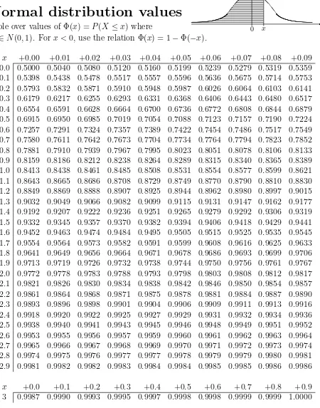
Normal distribution values

✻

✲ ✓

✓ ❙❙

x

0 Φ(x)

Table over values of Φ(x) =P(X _≤x) where

X _∈N(0,1). For x <0, use the relation Φ(x) = 1₋Φ(₋x).

x +0.00 +0.01 +0.02 +0.03 +0.04 +0.05 +0.06 +0.07 +0.08 +0.09 0.0 0.5000 0.5040 0.5080 0.5120 0.5160 0.5199 0.5239 0.5279 0.5319 0.5359 0.1 0.5398 0.5438 0.5478 0.5517 0.5557 0.5596 0.5636 0.5675 0.5714 0.5753 0.2 0.5793 0.5832 0.5871 0.5910 0.5948 0.5987 0.6026 0.6064 0.6103 0.6141 0.3 0.6179 0.6217 0.6255 0.6293 0.6331 0.6368 0.6406 0.6443 0.6480 0.6517 0.4 0.6554 0.6591 0.6628 0.6664 0.6700 0.6736 0.6772 0.6808 0.6844 0.6879 0.5 0.6915 0.6950 0.6985 0.7019 0.7054 0.7088 0.7123 0.7157 0.7190 0.7224 0.6 0.7257 0.7291 0.7324 0.7357 0.7389 0.7422 0.7454 0.7486 0.7517 0.7549 0.7 0.7580 0.7611 0.7642 0.7673 0.7704 0.7734 0.7764 0.7794 0.7823 0.7852 0.8 0.7881 0.7910 0.7939 0.7967 0.7995 0.8023 0.8051 0.8078 0.8106 0.8133 0.9 0.8159 0.8186 0.8212 0.8238 0.8264 0.8289 0.8315 0.8340 0.8365 0.8389 1.0 0.8413 0.8438 0.8461 0.8485 0.8508 0.8531 0.8554 0.8577 0.8599 0.8621 1.1 0.8643 0.8665 0.8686 0.8708 0.8729 0.8749 0.8770 0.8790 0.8810 0.8830 1.2 0.8849 0.8869 0.8888 0.8907 0.8925 0.8944 0.8962 0.8980 0.8997 0.9015 1.3 0.9032 0.9049 0.9066 0.9082 0.9099 0.9115 0.9131 0.9147 0.9162 0.9177 1.4 0.9192 0.9207 0.9222 0.9236 0.9251 0.9265 0.9279 0.9292 0.9306 0.9319 1.5 0.9332 0.9345 0.9357 0.9370 0.9382 0.9394 0.9406 0.9418 0.9429 0.9441 1.6 0.9452 0.9463 0.9474 0.9484 0.9495 0.9505 0.9515 0.9525 0.9535 0.9545 1.7 0.9554 0.9564 0.9573 0.9582 0.9591 0.9599 0.9608 0.9616 0.9625 0.9633 1.8 0.9641 0.9649 0.9656 0.9664 0.9671 0.9678 0.9686 0.9693 0.9699 0.9706 1.9 0.9713 0.9719 0.9726 0.9732 0.9738 0.9744 0.9750 0.9756 0.9761 0.9767 2.0 0.9772 0.9778 0.9783 0.9788 0.9793 0.9798 0.9803 0.9808 0.9812 0.9817 2.1 0.9821 0.9826 0.9830 0.9834 0.9838 0.9842 0.9846 0.9850 0.9854 0.9857 2.2 0.9861 0.9864 0.9868 0.9871 0.9875 0.9878 0.9881 0.9884 0.9887 0.9890 2.3 0.9893 0.9896 0.9898 0.9901 0.9904 0.9906 0.9909 0.9911 0.9913 0.9916 2.4 0.9918 0.9920 0.9922 0.9925 0.9927 0.9929 0.9931 0.9932 0.9934 0.9936 2.5 0.9938 0.9940 0.9941 0.9943 0.9945 0.9946 0.9948 0.9949 0.9951 0.9952 2.6 0.9953 0.9955 0.9956 0.9957 0.9959 0.9960 0.9961 0.9962 0.9963 0.9964 2.7 0.9965 0.9966 0.9967 0.9968 0.9969 0.9970 0.9971 0.9972 0.9973 0.9974 2.8 0.9974 0.9975 0.9976 0.9977 0.9977 0.9978 0.9979 0.9979 0.9980 0.9981 2.9 0.9981 0.9982 0.9982 0.9983 0.9984 0.9984 0.9985 0.9985 0.9986 0.9986

x +0.0 +0.1 +0.2 +0.3 +0.4 +0.5 +0.6 +0.7 +0.8 +0.9 3 0.9987 0.9990 0.9993 0.9995 0.9997 0.9998 0.9998 0.9999 0.9999 1.0000

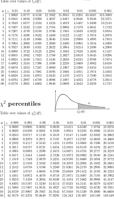
Percentiles:

α λα α λα

(8)

t

percentiles

✻

✲

tα(df) 0

α

Table over values of tα(df).

df α 0.25 0.10 0.05 0.025 0.02 0.01 0.005 0.001

1 1.0000 3.0777 6.3138 12.7062 15.8945 31.8205 63.6567 318.3088 2 0.8165 1.8856 2.9200 4.3027 4.8487 6.9646 9.9248 22.3271 3 0.7649 1.6377 2.3534 3.1824 3.4819 4.5407 5.8409 10.2145 4 0.7407 1.5332 2.1318 2.7764 2.9986 3.7470 4.6041 7.1732 5 0.7267 1.4759 2.0150 2.5706 2.7565 3.3649 4.0322 5.8934 6 0.7176 1.4398 1.9432 2.4469 2.6122 3.1427 3.7074 5.2076 7 0.7111 1.4149 1.8946 2.3646 2.5168 2.9980 3.4995 4.7853 8 0.7064 1.3968 1.8595 2.3060 2.4490 2.8965 3.3554 4.5008 9 0.7027 1.3830 1.8331 2.2622 2.3984 2.8214 3.2498 4.2968 10 0.6998 1.3722 1.8125 2.2281 2.3593 2.7638 3.1693 4.1437 12 0.6955 1.3562 1.7823 2.1788 2.3027 2.6810 3.0545 3.9296 14 0.6924 1.3450 1.7613 2.1448 2.2638 2.6245 2.9768 3.7874 17 0.6892 1.3334 1.7396 2.1098 2.2238 2.5669 2.8982 3.6458 20 0.6870 1.3253 1.7247 2.0860 2.1967 2.5280 2.8453 3.5518 25 0.6844 1.3163 1.7081 2.0595 2.1666 2.4851 2.7874 3.4502 30 0.6828 1.3104 1.6973 2.0423 2.1470 2.4573 2.7500 3.3852 50 0.6794 1.2987 1.6759 2.0086 2.1087 2.4033 2.6778 3.2614 100 0.6770 1.2901 1.6602 1.9840 2.0809 2.3642 2.6259 3.1737

χ

2

percentiles

✲ ✻

χ2_α(_df₎

0

α

Table over values of χ2

α(df).

(9)

Values of the Poisson distribuion

Table over values of F(x) =P(X _≤x) whereX _∈P o(λ).

λ 0 1 2 3 4 5 6 7 8 9 10 11 12 13

0.5 0.607 0.910 0.986 0.998 1.000 1.000 1.000 1.000 1.000 1.000 1.000 1.000 1.000 1.000 1 0.368 0.736 0.920 0.981 0.996 0.999 1.000 1.000 1.000 1.000 1.000 1.000 1.000 1.000 2 0.135 0.406 0.677 0.857 0.947 0.983 0.995 0.999 1.000 1.000 1.000 1.000 1.000 1.000 3 0.050 0.199 0.423 0.647 0.815 0.916 0.966 0.988 0.996 0.999 1.000 1.000 1.000 1.000 4 0.018 0.092 0.238 0.433 0.629 0.785 0.889 0.949 0.979 0.992 0.997 0.999 1.000 1.000 5 0.007 0.040 0.125 0.265 0.440 0.616 0.762 0.867 0.932 0.968 0.986 0.995 0.998 0.999 6 0.002 0.017 0.062 0.151 0.285 0.446 0.606 0.744 0.847 0.916 0.957 0.980 0.991 0.996

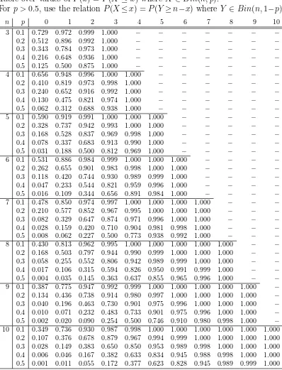
Values of the Binomial distribution

Table over values of P(x) =P(X ≤x) whereX ∈Bin(n, p).

Forp > 0.5, use the relationP(X_≤x) = P(Y _≥n₋x) whereY _∈Bin(n,1₋p).

n p 0 1 2 3 4 5 6 7 8 9 10

3 0.1 0.729 0.972 0.999 1.000 ₋ ₋ ₋ ₋ ₋ ₋ ₋ 0.2 0.512 0.896 0.992 1.000 ₋ ₋ ₋ ₋ ₋ ₋ ₋ 0.3 0.343 0.784 0.973 1.000 ₋ ₋ ₋ ₋ ₋ ₋ ₋ 0.4 0.216 0.648 0.936 1.000 ₋ ₋ ₋ ₋ ₋ ₋ ₋ 0.5 0.125 0.500 0.875 1.000 ₋ ₋ ₋ ₋ ₋ ₋ ₋ 4 0.1 0.656 0.948 0.996 1.000 1.000 − − − − − −

0.2 0.410 0.819 0.973 0.998 1.000 − − − − − −

0.3 0.240 0.652 0.916 0.992 1.000 − − − − − −

0.4 0.130 0.475 0.821 0.974 1.000 − − − − − −

0.5 0.062 0.312 0.688 0.938 1.000 − − − − − −

5 0.1 0.590 0.919 0.991 1.000 1.000 1.000 ₋ ₋ ₋ ₋ ₋ 0.2 0.328 0.737 0.942 0.993 1.000 1.000 ₋ ₋ ₋ ₋ ₋ 0.3 0.168 0.528 0.837 0.969 0.998 1.000 ₋ ₋ ₋ ₋ ₋ 0.4 0.078 0.337 0.683 0.913 0.990 1.000 ₋ ₋ ₋ ₋ ₋ 0.5 0.031 0.188 0.500 0.812 0.969 1.000 ₋ ₋ ₋ ₋ ₋ 6 0.1 0.531 0.886 0.984 0.999 1.000 1.000 1.000 ₋ ₋ ₋ ₋ 0.2 0.262 0.655 0.901 0.983 0.998 1.000 1.000 ₋ ₋ ₋ ₋ 0.3 0.118 0.420 0.744 0.930 0.989 0.999 1.000 ₋ ₋ ₋ ₋ 0.4 0.047 0.233 0.544 0.821 0.959 0.996 1.000 ₋ ₋ ₋ ₋ 0.5 0.016 0.109 0.344 0.656 0.891 0.984 1.000 ₋ ₋ ₋ ₋ 7 0.1 0.478 0.850 0.974 0.997 1.000 1.000 1.000 1.000 − − −

0.2 0.210 0.577 0.852 0.967 0.995 1.000 1.000 1.000 − − −

0.3 0.082 0.329 0.647 0.874 0.971 0.996 1.000 1.000 − − −

0.4 0.028 0.159 0.420 0.710 0.904 0.981 0.998 1.000 − − −

0.5 0.008 0.062 0.227 0.500 0.773 0.938 0.992 1.000 − − −

(10)

Trigonometrics

The Fourier transform ofg The inverse Fourier transform of G