M – 29
ESTIMATION OF LOGISTIC SMOOTH TRANSITION AUTOREGRESSIVE
MODEL USING GENETIC ALGORITHM
Meiliyani Siringoringo, Irhamah
Departement of Statistics, Institut Sepuluh Nopember Surabaya
Abstract
Time series data not only create linear model but also nonlinear model, especially in the economic. One of nonlinear model in time series is smooth transition autoregressive (STAR). STAR model is the development of Self-Exciting Autoregressive (SETAR) model with two regimes. STAR smoothen the SETAR two regimes with a transition function and one of that is logistic function which then form LSTAR models (logistic smooth transition autoregressive). After, determining order p and delay d, estimation of π1, π2,γ and c using genetic algotihm. By GA (genetic algorithm), that is a technique to search for solutions with various combinations of genes in a chromosome in order to obtain a global optimum solution, . Evaluation of chromosomes carried by the fitness function through procedures such as selection, crossover and mutation. Application of genetic algorithm (GA) will be conducted to identify the data model of LSTAR on stock return are included in the LQ 45 index that show LSTAR with GA better than AR model.
Key words: genetic algorithm, nonlinear, stock return, LSTAR
INTRODUCTION
The SETAR (Self-Excited Threshold Autoregressive) model assumes that the border between the two regimes is given by a specific value of threshold variabel. Amore gradual transition between the different regimes can be obtained by replacing the indicator function by a continous function, which changes smoothly from 0 to 1. The resultant model is called a Smooth Transition Autoregressive (STAR) model (van Dijk & Franses, Nonlinear Time Series Models in Empirical Finance, 2003). Continous function is called also transition function, one of the transition function is logistic function so the model become logitic STAR (LSTAR). As
RESEARCH METHOD
Logistic Smooth Transition Autoregressive
Generalization of nonlinear two-regime univariate self-exciting threshold
autoregressive, SETAR model, so as to make the transition from one regime to the other smooth, that is, STAR model (Lukkonen, Saikkonen, & Terasvirta, 1988). Consider the
following STAR model of order p
' '
10 1 20 2 Z ; ,
t t t t d t
Z
π w
π w F
c u (1)where ut nid 0,
2
, πj
j1,...,jp
',
' 1
1, 2, t t ,..., t p
j w Z Z and F is a transition
function which by convention is bounded by zero and one. If the the transition function is logistic function
1Z
t d; ,
1 exp
t d,
0
F
c
Z
c
(2)Model (1) with (2) is called the logistic STAR (LSTAR). When
, model (1) with (2) becomes a TAR(p) and when
0 becomes a linear AR(p) model (Terasvirta & Anderson, Characterizing Nonlinearitas in Business Cycles Using Smooth Transition Autoregressive Models, 1992).Before modelling the LSTAR model, we must testing the linearity using terasvirta test. Terasvirta test is a Lagrange Multiplier-type that is based on neural network model where null hypothesis show that the data is linear and the alternative show that the data is nonlinear (Terasvirta, Lin, & Granger, Power of The Neural Network Linearity Test, 1993). Then the analysis will proceed with model identification, estimation and testing parameters, diagnostic testing and forecasting.
It is important in nonlinear time series is to determine whether a linear model or qualified enough to represent the data generation process. LSTAR model identification is to determine the order p and the delay d. LSTAR model follow AR process so lenght of order p
can be obtained by looking at ACF plot. The general technique to choose the appropriate lag is to use selection criteria such as AIC or SBIC (van Dijk, Terasvirta, & Franses, Smooth Transition Autoregressive Models - A Survey of Recent Developments, 2002).
Determining delay d in transition variable by computing LM3 statistics for various
candidate transition variables
s
1t,...,
s
mt, say, and selecting the one for which the LM3 of thetest is highest or p-value of the test is smallest. After we find orde p and d, parameter estimation (1) will be computed by GA by minimizing SSE that is [6]
21
T
t t
t
Z
Z
(3)Genetic Algorithm (GA)
An algorithm is a series of steps for solving a problem. A genetic algorithm is a problem solving method that uses genetics as its model of problem solving. It’s a search technique to find approximate solutions to optimization and search problems (Sivanandam & Deepa, 2008).
are applied directly on the chromosomes, and are used to perform mutations and recombinations over solutions of the problem. Appropriate representation and reproduction operators are really something determinant, as the behavior of the GA is extremely dependant on it. Frequently, it can be extremely difficult to find a representation, which respects the structure of the search space and reproduction operators, which are coherent and relevant according to the properties of the problems (Sivanandam & Deepa, 2008).
Selection is supposed to be able to compare each individual in the population. Selection is done by using a fitness function. Each chromosome has an associated value corresponding to the fitness of the solution it represents. The fitness should correspond to an evaluation of how good the candidate solution is. The optimal solution is the one, which maximizes the fitness function. Genetic Algorithms deal with the problems that maximize the fitness function. But, if the problem consists in minimizing a cost function, the adaptation is quite easy. Either the cost function can be transformed into a fitness function, for example by inverting it; or the selection can be adapted in such way that they consider individuals with low evaluation functions as better. Once the reproduction and the fitness function have been properly defined, a Genetic Algorithm is evolved according to the same basic structure. It starts by generating an initial population of chromosomes. This first population must offer a wide diversity of genetic materials. The gene pool should be as large as possible so that any solution of the search space can be engendered. Generally, the initial population is generated randomly (Sivanandam & Deepa, 2008).
Then, the genetic algorithm loops over an iteration process to make the population evolve. Each iteration consists of the following steps:
1. Selection: the first step consist in selecting individuals for reproduction. This selection is done randomly with a probability depending on the relative fitness of the individuals so that best ones are often choosen for reproduction than poor ones.
2. Reproduction: In the second step, offspring are bred by the selected individuals. For generating new chromosomes, the algorithm can use both recombination and mutation. 3. Evaluation: the fitness of the new chromosomes is evaluated.
4. Replacement: during the last step, indviduals from the old population are killed and replaced by the new ones (Sivanandam & Deepa, 2008).
The steps of analysis to identification and estimation LSTAR model are as follows: 1. Testing nonlinearity.
2. Determine lenght of order p and delay d that show nonlinierity.
3. GA process to find the best model for LSTAR using conditional least square as estimation
method for πj
j1,...,jp
'. Roullete wheel for the selection and for the reproduction will be used crossover and mutation.RESULT AND DISCUSSION
The GA proposed in this study is used to find parameters of the LSTAR model. First of all, will be used simulated data modeled LSTAR (2,1) in estimating model parameters. After that, the estimated parameters using the GA will be apllied to the data stock return of.
For the simulation of data, will be generated 500 sample. Consider the LSTAR (1,1) model as given as follows:
0.3 0.5 1
1
0.1 0.5 1
t t t d t t d t
where
1 1
1 exp
5
t d t
F Z
Z
dan ut nid 0, 0.25
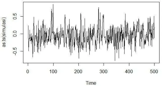
(van Dijk & Franses,Nonlinear Time Series Models in Empirical Finance, 2003). Graphic illustration in the form of a time series plot and plot the data with a lag of one of the result of the simulation is shown in Figure 1.
Figure1. Time Series Plot of the Simulation
Figure 1 show that the data is stasionary. It shown that the time series data lies around 0. And the results of estimation parameter using GA is presented in Tabel 1.
Table 1. Estimation parameter simulation LSTAR(1,1) model using GA
Parameter Estimasi
π01 -0.2668
π11 -0.45
π02 0.0932
π21 0.45
γ 4.5
c -0.00001
The GA estimation has the smallest SSE that is 29.4228. After that, will be estimate parameter of the data that have generated with AR(1). We find SSE that is 31,1486 with the parameter estimation presented in Table 2.
Table 2. Estimation parameter simulation AR(1)
Parameter Estimasi
π01 -0.0355
π1 0.2907
π2 -0.0434
Application of parameter estimation LSTAR using GA will use the stock return data of BBRI. Figure 1 show time series plot of stock return BBRI.
Figure 2. Time Series Plot of Stock Return BBRI
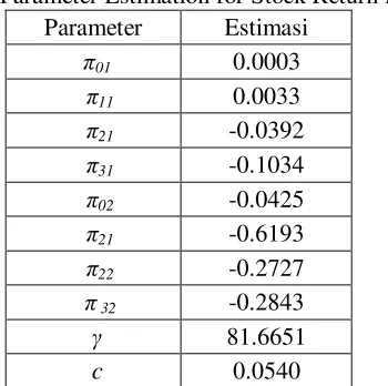
From stock return BBRI data, testing linearity using Terasvirta test show that the data is nonlinear. The data follow AR(3) with delay d is 1. The fitness function is SSE where GA process will minimize SSE to find the best solution. The result of estimation parameter using GA for stock return BBRI is presented in Table 3.
Tabel 3. Parameter Estimation for Stock Return BBRI
Parameter Estimasi
π01 0.0003
π11 0.0033
π21 -0.0392
π31 -0.1034
π02 -0.0425
π21 -0.6193
π22 -0.2727
π 32 -0.2843
γ 81.6651
c 0.0540
From parameter estimation of LSTAR(3,1) for stock return BBRI, GA process find the best solution with SSE is 0.5954.
2
1 2 3 1
1 3 1
0.0003 0.0033
0.0392
0.1034
0.0425 0.6193
0.2727
0. 8
1
2 43
t
t t t t t
t t t t
Z
Z
Z
Z
F Z
Z
Z
Z
F Z
u
(5)
where
1 1
1 exp
81.6651
0.0540
t d t
F Z
Z
For comparison, the stock return BBRI data will be modeled with AR. And the best fitted AR model is AR(3) with SSE 0,6006.
1 2 3 1
0, 001 0, 0259 0.0849 0.0230 1.156
t t t t t t
CONCLUSION AND SUGGESTION
This study show that GA can be used to estimate parameter of LSTAR. Parameter estimation using GA for stock return BBRI data is better than AR becuase LSTAR-GA produces SSE less than AR. Determining population size, we must consider the interval of parameter especially for real-valued encoding that can reach all possibilty or combination of the gene or solution.
REFERENCES
Lukkonen, R., Saikkonen, P., & Terasvirta, T. (1988). Testing Linearity Againts Smooth Transition Autoregressive Models. Biometrika, 75 (3), 491-9.
Sivanandam, S. N., & Deepa, S. N. (2008). Introduction to Genetic Algorithms. New York: Springer.
Terasvirta, T. (1994). Specification, Estimation and Evaluation of Smooth Transition
Autoregressive Models. Journal of the American Statistical Association, 89 (425), 208-218.
Terasvirta, T., & Anderson, H. M. (1992). Characterizing Nonlinearitas in Business Cycles
Using Smooth Transition Autoregressive Models. Journal of Applied Econometrics, 7.
Terasvirta, T., Lin, C. F., & Granger, C. W. (1993). Power of The Neural Network Linearity Test. Journal of Time Series Analysis, 14.
van Dijk, D., & Franses, P. H. (2003). Nonlinear Time Series Models in Empirical Finance.
New York: Cambridge University Press.
van Dijk, D., Terasvirta, T., & Franses, P. H. (2002). Smooth Transition Autoregressive Models -