and Information Processing Vol. 1, No. 3 (2003) 243–261
c
World Scientific Publishing Company
THRESHOLDING WAVELET NETWORKS FOR SIGNAL CLASSIFICATION
NEMUEL D. PAH∗and DINESH KANT KUMAR
RMIT University, Melbourne, Australia
∗[email protected] Received 25 October 2002
This paper reports a new signal classification tool, a modified wavelet network called Thresholding Wavelet Networks (TWN). The network is designed for the purposes of classifying signals. The philosophy of the technique is that often the difference between signals may not lie in the spectral or temporal region where the signal strength is high. Unlike other wavelet networks, this network does not concentrate necessarily on the high-energy region of the input signals. The network iteratively identifies the suitable wavelet coefficients (scale and translation) that best differentiate the different signals provided during training, irrespective of the ability of these coefficients to represent the signals. The network is not limited to the changes in temporal location of the signal identifiers. This paper also reports the testing of the network using simulated signals.
Keywords: Wavelet networks; neural networks. 1. Introduction
Pattern recognition and classification of signaland data are essentialfor our com-puterised society for automating the process of identifying a person, an object or an event. Pattern recognition consists of at least three phases: feature extraction, feature selection and classification.1
Feature extraction gives condensed representation of the input signal. Appro-priate representation of the signalmust contain allthe important features that can be used to discriminate the signalpattern from the other signals. The purpose of representation is to reduce the complexities of the signal, while highlighting the properties that are suitable to recognize the pattern. Feature extraction involves transforming the signal while maintaining its completeness. The transformed data contain discriminative and other information. Selection of the transformation to be used is determined by initialknowledge of the discriminative pattern and space of the transformation.
To make the process of recognition more efficient, it is necessary to select suitable features that best identify the different patterns. Feature selection phase is necessary to separate the meaningfulfeatures that can best represent the input pattern with
244 N. D. Pah & D. K. Kumar
minimum redundancy. The optimisation of the feature selection is controlled by its cost function.
The classification phase is the process to modify and map the selected features to the desired output format.
The development of Wavelet Transform has opened more opportunities in signal classification. Wavelet transform provides the temporal and spectral perspectives. It also provides the flexibility of choice of a wide variety of wavelet functions with properties well matched with the signal.
Wavelet transform has been widely used in the computation of many signal properties such as instantaneous frequency, detection of singularities, regularity measurement and fractalstructures.2–11All these properties are significant in order
to determine patterns of a class of signal.
The flexibility offered by the wavelet transform comes at the cost of having to select or adjust several number of input parameters. For suitable representation, the wavelet function, range of scale and translation have to be selected properly. This requires either prior knowledge of the signal and wavelet properties or exper-imentally determining the most suitable parameters. The latter is difficult due to computationalcomplexity.
To overcome the problem, the efficacy of neural networks has been combined with wavelet transforms to generate wavelet networks.1 The wavelet networks can
generate wavelet coefficients iteratively to represent and classify the input signal. In the past few years, many types of wavelet networks have been introduced. Most of the wavelet networks are designed for the purpose of function approximation.12–24
Some researchers1,25–32 have attempted to use the combination of
neuralnet-works with wavelet transforms to directly classify the signal. The input signal is classified by iteratively locating the positions in wavelet’s time-scale space that best discriminate the input patterns. The inconsistent temporalalignment of the important events in the input signals often creates problem for this classification technique.
This paper reports our efforts to develop a new wavelet network that can over-come the limitations of previous wavelet networks. This wavelet network introduces an upper-lower thresholding process that allows the network to select the suitable wavelet coefficients based on signal properties. The selection is not depending on the temporalalignment of the coefficients.
This paper is organised into six sections. Section 2 reviews the basic concept of wavelet transform while Sec. 3 reviews the different types of wavelet networks. Section 4 presents the proposed thresholding wavelet network. Section 5 presents the simulation of the network, while Sec. 6 concludes the paper.
2. Wavelet Transform
Wavelet transform of a functionf ∈L2(R) is defined as the correlation betweenf
W f(u, s) =f, ψ∗u,s, (1)
The magnitude of wavelet coefficient|W f(u, s)|will be higher if the properties of the functionf in the neighbourhood oft=umatch the properties of the wavelet function ψ∗
u,s at scale s. By selecting a wavelet function with a certain proper-ties (temporal or spectral), one can extract the portion of the analysed signal that match the properties of the wavelet function being used. The magnitude of wavelet coefficients contains information related to certain properties in the analysed sig-nalsuch as the instantaneous frequency and regularity.2,4The maxima of wavelet
transform can also be used to approximate signal as well as removing noises.2,33,34
2.1. Instantaneous frequency
Wavelet transform can measure time-frequency variation of spectral components with a non-constant time frequency resolution.2 The time-frequency atom of a wavelet function varies according to scales. A wavelet atom
ψu,s(t) =√1 is centred att=uwith time spreading proportionalto scales. In frequency domain, the atom is centred atη/swith a size proportionalto 1/s. The centre frequency at scales= 1 is defined as:
The ability of wavelet atom to increase its time resolution in high frequency, and increase its frequency resolution in low frequency makes it able to follow the rapid change in spectralcomponent with good resolution.
The instantaneous frequency can be detected from the ridges2 of normalised
scalogram:
The ridges (u, ξ(u)) are the maxima points at each translationu. The magnitude of the normalised scalogram (5) corresponds to the amplitude of the particular spectral components. If the coefficients were calculated using analytic wavelet, the phase and amplitude information of the analysed signal are well separated.
2.2. Regularity measurement
Most signals are characterised by their regularity pattern.2Wavelet coefficients can
246 N. D. Pah & D. K. Kumar
A function f is pointwise Lipschitzα≥0 att=ν if there exist K >0, and a polynomialpm of degreem=⌊α⌋such that:
|f(t)−pν(t)| ≤K|(t−ν)|α. (6) Wavelet transform estimates the Lipschitz exponent α by using wavelet with n=⌈α⌉ vanishing moments. The wavelet transform of the function f =pm+eν only depends on the singularity eν since a wavelet with n vanishing moments is orthogonalto any polynomialof degreem≤n−1.
W f(u, s) =W eν(u, s). (7)
Lipschitz regularity is related to the decay of the magnitude of wavelet coef-ficients |W f(u, s)| and the singularity point is located by finding the abscissaν where wavelet modulus maxima converge to at the finest scale.
The global singularity of a signal with many non-isolated singularities can also be measured from the decay of wavelet modulus maxima.
2.3. Maxima of wavelet coefficients
Sections 2.1 and 2.2 show that the location and the magnitude of wavelet transform maxima carry information related to the spectralcomponent of the signalas well as its singularities. Wavelet modulus maxima at scale s0 is defined as any points
(u0, s0) such that|W f(u0, s0)| satisfy:
∂W f(u0, s0)
∂u = 0. (8)
By modifying wavelet maxima, one can approximate a signal at different level of approximation, remove noises or extract part of the signalthat relates to specific category. Thresholding wavelet coefficients can effectively select the way a signal is going to be approximated for a specific purpose.
3. Wavelet Networks
A wavelet network is a class of neural networks that combines wavelet trans-form with neuralnetwork algorithm.1This combination provides a toolto perform
wavelet transform analysis in a parallel, adjustable and able-to-learn fashion. Wavelet transform calculates the correlations between f and wavelet function ψ at various different combination of translation and scale (u, s). The calculation can be faster if it is done in parallel computation, where each unit calculates only one wavelet coefficient.
There are many different types of wavelet networks. In general they can be grouped into two major streams1: approximation wavelet networks and classification
wavelet networks.
3.1. Approximation wavelet networks
Approximation Wavelet Network (AWN)12–24is based on nonlinear wavelet
approx-imation. The nonlinear approximation of a functionf fromM wavelet coefficients indexed with IM is defined as2:
fM =
(j,n)∈IM
f, ψ(j, n)ψ(j, n). (9)
The selection of the set of wavelet coefficients{(j, n)m}m∈IM is generally based on the effort to minimise the approximation error:
ǫ[M] =f−fM 2 . (10)
A small approximation error can be achieved with a minimal number of wavelet coefficients if the transformation uses orthogonalwavelets. However, if the network can maintain the reduction of error and redundancy, it is not necessary to use orthogonal wavelets. Non-orthogonal wavelets are needed especially in analysing signals with many non-isolated singularities. It is also possible to use different type of wavelets in one network to approximate the functionf. In this case the wavelet functions are most likely to be non-orthogonal.
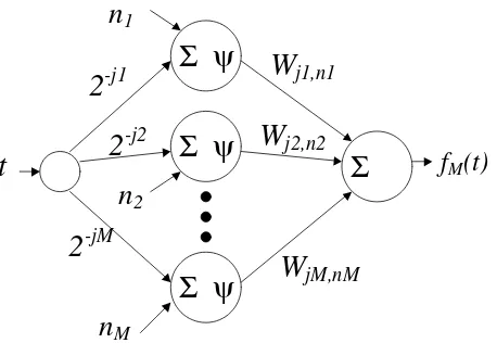
An AWN is commonly implemented as three layers neural network. The output layer has only one node with a linear transfer function. The hidden layer has M wavelet nodes with the wavelet function as their transfer function.
fM =
The wavelet coefficients are represented by weighting factorsWj,nbetween hid-den and output layer.
Wj,n≈ f, ψj,n. (12)
The weighting factor of the hidden nodeswhdetermines the scale of the wavelet function while its bias bh determines the time translation.
Wh={2jh
}h=1,2,...,M and bh={nh}h=1,2,...,M. (13) Bias of output nodeb0is necessary to approximate function with non-zero
248 N. D. Pah & D. K. Kumar
Σ ψ
Σ ψ
Σ ψ
t
2
-j12
-j22
-jMn
1n
2n
MΣ
W
j1,n1W
j2,n2W
jM,nMf
M(t)
Fig. 1. The architecture of approximation wavelet networks.
approximates the functionf. Some of the learning algorithms that have been used in the optimisation of the parameters are gradient descent,18,19,23,24,34 competitive
learning,35dyadic selection,12evolutionary computation36and genetic algorithm.37
The number of wavelet nodesM can be optimised by using an algorithm such as competitive learning.
Like all approximation processes, the wavelet network optimises its parameters by minimising the energy of its error ε[M]. The selection of wavelet coefficient is therefore, based on the coefficients magnitude. The network tends to prioritise high-energy regions of f. If the approximationfM is to be used in classification purposes, it is only effective if the deterministic factors are immersed in the high-energy regions of the signal. There are number of natural signals where this may not be the case.
3.2. Classification wavelet networks
Classification Wavelet Network (CWN)1,25–32 uses neuralnetworks algorithm to
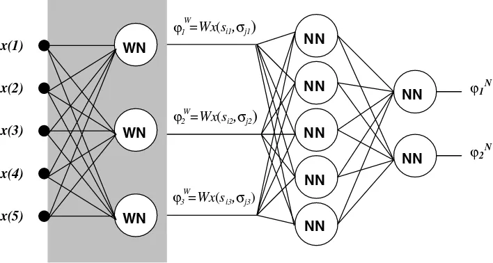
select the locations of wavelet coefficient (u, s) that are reliable for categorising the input signals. The CWN, as shown in Fig. 2, can be seen as a neural network, which the first layer consists of wavelet nodes followed by some neural network layers. The wavelet layer acts as a feature extraction layer while the neural network layers are for feature selection and classifier.
The output of each wavelet nodeϕW is defined as the inner product of the input signalf and a wavelet function at a specific time-scale ψu0,s0. The output ϕ
W is actually a wavelet coefficient at scales0 and translationu0.
ϕW0 =f, ψu0,s0=W f(u0, s0). (14)
NN
Fig. 2. The architecture of classification wavelet networks. The first layer consists of wavelet nodes which calculates wavelet coefficients of the input x(n). The subsequent layers are neural network layers.
and weighting factorswand biasb. ϕN =fT
During the learning phase, the parameters of wavelet nodes u and s and the weights and biases of the neuralnetwork’s nodes are adjusted by backpropagating the error of the neural network. The learning process of each wavelet node can be seen as the movement of a wavelet’s Heisenberg box in time-scale space from its initialposition (ui, si) to its optimum position (u0, s0) as shown in Fig. 3.
The number of nodes in wavelet layer K determines the number of wavelet Heisenberg boxes. The number of nodesKas well as the initial value of the param-eters (ui, si) have to be selected carefully for a specific classification problem. The selection of initial value is significant to ensure that the nodes are not overlapping each other during the learning phase.
There are two main disadvantages of this wavelet networks; temporal depen-dence of classification and lack of optimisation for classification. The resultant net-work have fixed spots in time-scale space{(un, sn)}n=1,2,3,...,K. Consequently, the
250 N. D. Pah & D. K. Kumar
u
u
1u
4u
2u
3η
/s
4η
/s
3η
/s
2η
/s
1f
Fig. 3. Learning process in each wavelet nodes is illustrated as the movement of a wavelet Heisen-berg box from initial position (ui, si) to its optimum position (uo, so).
The second disadvantage is that this network forces the subsequent neuralnet-work layers to classify input signal based only on the values of the wavelet co-efficients W f(u, s). Processing of these coefficients before classification may help optimise the classification process and overcome these problems.
4. Thresholding Wavelet Networks
To overcome the above disadvantages of wavelet networks in classifying non-stationary, semi-random signals, a new type of wavelet network called Thresholding Wavelet Network (TWN) has been designed. Wavelet thresholding has been widely used in the past in wavelet signal estimation and de-noising.33,38
The TWN, reported in this paper, uses wavelet thresholding in a different ap-proach. The TWN was designed for classification purpose. This network selects the wavelet nodes based on the thresholding of the local maxima in each of the scale bands of the Continuous Wavelet Transform (CWT).
Wavelet maxima are the wavelet coefficients that satisfy Eq. (8). In discrete domain this zero derivative is nearly impossible. For that reason, wavelet maxima are selected where the partial derivation changes sign from positive to negative.
The wavelet maxima are thresholded at the thresholding layer. This process selects the wavelet maxima based on their magnitude in relation to the thresholding levels. Maxima with magnitude less than the thresholding level are removed while maxima with higher magnitude are propagated.
xs=ηs(x, θ)sgn(x)(|x| −θ)+, (16)
whereθ >0 is the threshold, while hard thresholding ofxis defined as:
xh=ηh(x, θ) =
x for|x|> θ ,
0 for|x| ≤θ . (17)
4.1. The significance of thresholding
Most signals can be characterised by the occurrence of transients such as QRS-complex in electrocardiography and motor unit action potential (MUAP) in electromyography.39These transients can be characterised by their properties such
as magnitude, frequency distribution, regularity and polynomial degree. It is impor-tant to use these features for the classification of such signals. Wavelet transform can be used to measure the spectral content, transients, regularity and polynomial degree of a signal while thresholding extracts these features with respect to the specific magnitudes and thus are an obvious choice.
To classify the signals, the occurrence of these transients must be detected and analysed. The temporal locations of the transients are often not necessary in the classification. By thresholding the wavelet coefficients, the temporal location may be lost but the features related to the occurrence of the events are extracted.
It is known that the position of wavelet coefficients maxima stores information about the frequency and singularity point. The question will be, what information is stored in the magnitude of these maxima?
The magnitude of wavelet coefficients |W f(u, s)|are related to the magnitude of spectralcomponents in the analysed signalf. Suppose:
f(t) =a(t) cosφ(t), (18)
wherea(t) is the amplitude andω(t) =φ′(t) is instantaneous frequency.
The amplitude a(t) recovered from wavelet coefficients when using a nearly analytic waveletψ(t) =g(t)eiηt is calculated as
a(u) = 2
s−1|W f(u, s)|2
|g(0)ˆ | , (19)
whereu=t−t0is the time shift and ˆg(0) is the Fourier transform of window g(t)
atω= 0. If the coefficients are not calculated with analytic wavelet the magnitude and phase are not well separated. However, the magnitude of wavelet coefficients are still related to the spectral amplitudea(t).
a(t−t0)∝ |W f(u, s)|. (20)
252 N. D. Pah & D. K. Kumar
The magnitude of wavelet coefficients is also related to the energy of signal with specific singularity. Equations (21)–(24) examine this relationship. Regularityαis measured from the decay of wavelet coefficients towards finest scale.
α∝lim the neighbourhood of the pointt=ν, then
|W f(u, s)| ≤Ksα+1/2. (22) The magnitude of wavelet coefficient att=uat a specific scales0, is related to
the energy of the signalin the temporalregion of the singularity. Suppose a function f has regularityαatt=ν, the functionf can be approximated with a polynomial of degree n = ⌊α⌋ and an error function ε: f = pν +εν. If the function is then amplified by a factor ofA, its wavelet coefficient att=ν will also be amplified by the same amount.
By thresholding the coefficient, the portion of the input signal with a specific singularity at certain amplification can be selected.
Thresholding of wavelet coefficients has numerous applications. One of the appli-cations is signaldenoising.33Denoising is a process of estimating a class of function
from its corrupted version. It is based on the assumption that the energy of the uncorrupted function is concentrated in a small number of coefficients while the noise is spreading over a large number of wavelet coefficients.34 Ifdrepresents the
corrupted version of the originalsignalf ∈[0,1], it is expressed as:
di=f(ti) +σzi fori= 1,2,3, . . . , n−1. (25) The noise zi iid∼ N(0,1) is approximated by an independent and identically distributed Gaussian function of levelσ.
The other assumption is that the energy of noise is less than the energy of the uncorrupted function. For this reason, de-noising process is often interpreted as optimising the mean squared error (Edi−fi2)/nof the estimation.
a classification process must include upper–lower threshold to select the coefficients belonging to the middle range energy. The upper–lower thresholding function is defined as:
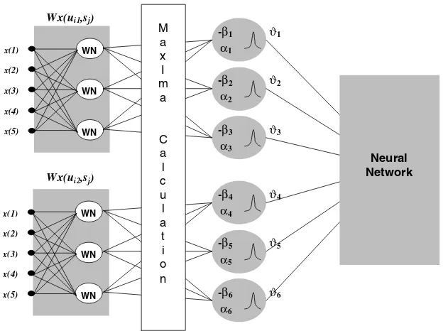
Thresholding wavelet networks consist of four blocks of network layer: a wavelet layer, maxima layer, thresholding layer and neural networks layers (Fig. 4). The input signal is applied to the wavelet layer. The input to the thresholding layer is the wavelet maxima at each scale of interest. The thresholds (θl, θh) for all maxima corresponding to one scale are the same. The scale-dependent-threshold allows the network to distinguish between scales based on magnitude. The output of wavelet thresholding nodeϕis the number of wavelet maxima with magnitude between θl andθh.
N is the number of wavelet maxima for that particular scales, whil eηT is the thresholding function. The output of the thresholding node is the number of wavelet maxima with magnitude betweenθlandθh. The output of threshold functionηT in Eq. (27) equals to one if its input is betweenθlandθhand equals to zero otherwise.
xT =ηT(x, θl, θh) =
1 forθl< x < θh,
0 forx≤θl orx≥θh. (28) This thresholding function also has to be a continuous function so that the derivative of the function exists. Thus, a Gaussian function g(x) =e−x2
was used as the thresholding function as below:
xT =ηT(x) =e−α2(x−β)2. (29) The output of the thresholding node is:
ϕ=
The biasβ determines the centre of g(x) whil eαdetermines the width of the function. The combination ofαandβ determines the upper and lower thresholds. Figure 5 illustrates the thresholding wavelet node.
254 N. D. Pah & D. K. Kumar
Fig. 4. A thresholding wavelet network. The network has six thresholding nodes (three for each scale).
Fig. 5. The wavelet thresholding node.
4.3. Learning process
these parameters were changed to reduce the classification error. The network was using a supervised learning algorithm. In the supervised learning algorithm, the network’s parameters are adjusted to properly relate the inputs f(t) and target outputϕT provided in the training set{(f1(t), ϕT1),(f2(t), ϕT2), . . . ,(fn(t), ϕT n)}.
In each thresholding node, the learning is the process to locate the lower and upper threshold levels (θl and θl) of each node. Determining the optimum value of the threshold parameters ensures number of wavelet coefficients with magnitude θl≤ |W f(u, s)| ≤θh can best categorise the class of input signals.
There are many algorithms currently available that can be used to optimising these parameters. The TWN reported in this paper was using the gradient descent algorithm. In gradient descent algorithm, the parameters are optimised to the neg-ative direction of partialderivation of its cost functionSSE to each parameter.
αnew=αold−ρ
The cost functionSSE is defined as the sum-squared of the difference between target outputϕT and the actualoutputϕ.
E= 1
2(ϕT −ϕ)
2. (33)
The amount of change in each iteration is determined by the partialderivation of the cost function and a learning rate coefficientρ.
The partialderivations of the cost function are: ∂SSE The learning process is repeated until the sum-squared-errorSSE falls below a predefined maximum errorET. At this stage the network is considered as able to classify the training pattern with an error less thanET.
5. Network Simulation
An experiment was conducted to determine the ability of this network to classify simulated signals. There were 160 simulated signals created for the experiments. The length of each signal was 1,000 samples. These signals had the following properties: (1) Consists of number of transients representing the current distribution of muscle
fibre action potential(MUAP),Im.40,41
256 N. D. Pah & D. K. Kumar
(2) The signals represent two classes each of 80 signals.
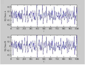
(3) Signals in class A (Fig. 6(a)) consist of 100 transients of magnitude 0.1 and 100 transients of magnitude of 0.04. These transients were located randomly. (4) Signals in class B (Fig. 6(b)) were very similar to signals belonging to class
A. These signals consist of 100 transients of magnitude 0.1, 100 transients of magnitude of 0.04 and 10 transients of magnitude 0.07. These transients were located randomly.
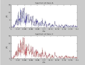
The difference between the two classes was not observable in the plot of the sig-nals (Fig. 6) as well as in their spectrum (Fig. 7) since the difference was determined by a small (10) number of transient with a low amplification.
The proposed thresholding wavelet network was simulated using graphic user interface of Matlab 6.1 as shown in Fig. 8. 40 signals of each class were used to train the network. These signals were scaled by a factor of 100 before being applied to the network to avoid quantisation error in the network calculation.
The training process was recorded in Fig. 8. It was observed that after 200 epochs theSSE of the network drops from about 10 to 0.1. The graphs on top-left
Fig. 6. (a) A signal of Class A consists of 100 waveImwith gain of 0.1 and 100 waveImwith
Fig. 7. The spectrum of simulated signals from Class A and B.
and bottom-left corner of Figure 11 show that the biases (β) of thresholding wavelet nodes converged to four values (or ranges): 0.3, 0.59–0.66, 0.91–0.92, and 1.3 and four of these converged to one point 0.91–0.92. It can also be observed that the four nodes that converge to a common value have higher weights (α) and thus have narrower thresholding function.
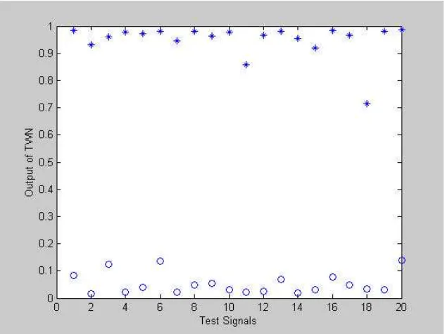
After completing the training process, the network was tested using the 40 test signals. The results are presented in Fig. 9. The signals that belongs to group A are marked with “o” while that of group B are marked with “*”. From the figure it is observed that the wavelet network is able to converge the thresholding values to best classify the signals and in this example, 100% classification is achieved.
6. Conclusion
This paper presents a new type of wavelet network, the Thresholding Wavelet Net-work. It is designed for the purpose of classifying signals based on the magnitude of wavelet maxima.
258 N. D. Pah & D. K. Kumar
Fig. 8. The learning process of thresholding wavelet network. The network is trained to classify 2 groups of signals (see Fig. 9) each consists of 20 signals. From top left corner clockwise: The thresholding functions of eight nodes after 200 epochs; the recording of SSE of the entire network; the recording of learning rate; the recording of bias of each thresholding nodes which indicates the centre of the thresholding function.
process to select wavelet maxima with certain magnitude that characterised the input signals.
The paper reports the simulation and testing of the network and the results are extremely promising. The results demonstrate several advantages of thresholding wavelet networks.
(1) It classifies the signals irrespective of the difference being in the low or high-energy region of the signal.
(2) It can extract the features of transients occurs in a signal.
(3) It is dynamic and classification is not affected by the change in temporal loca-tion of the event.
This network has to be tested with realsignals to determine the efficacy of the network. One shortcoming of this network is that the scale and wavelet basis function are invariant. The authors intend to include selection of scale and wavelet basis in its learning process.
References
1. H. Dickhaus and H. Heinrich,Classifying biosignals with wavelet networks, inIEEE Engineering in Medicine and Biology(IEEE, 1996), pp. 103–111.
2. S. Mallat,A Wavelet Tour of Signal Processing. 1999, London(Academic Press, 1999). 3. W.-L. Hwang and S. Mallat, Characterization of Self-Similar Multifractals with Wavelet Maxima1993, Courant Institute of Mathematical Sciences, Computer Science Department, New York University, pp. 1–25.
4. S. Mallat and W. L. Hwang, Singularity detection and processing with wavelets, in IEEE Transaction on Information Theory38(2) (1992) 617–643.
5. A. Arneodoet al.,Singularity spectrum of multifractal function involving oscillating singularities, inJ. Fourier Anal. Appl.4(2) (1998) 159–174.
6. P. Goncalves, R. Reidi and R. Baraniuk, Asimple statistical analysis of wavelet-based multifractal spectrum estimation, INRIARocquencourt (1998) pp. 1–5.
7. J. F. Muzy, E. Bacry and A. Arneodo, The multifractal formalism revisited with wavelets, inInt. J. Bifurcation Chaos4(2) (1994) 245–302.
8. F. H. Y. Chanet al., Multiscale characterization of chronobiological signals based on discrete wavelet transform, inIEEE Trans. Biomedical Engrg. 47(1) (2000) 88–95. 9. J. Y. Thamet al., Ageneral approach for analysis and application of discrete
multi-wavelet transform, inIEEE Trans. Signal Processing48(2) (2000) 457–464.
10. I. W. Selesnick, Balanced multiwavelet bases based on symmetric FIR filters, inIEEE Trans. Signal Processing48(1) (2000) 184–191.
11. S. Karlsson, J. Yu and M. Akay,Time-frequency analysis of myoelectric signals during dynamic contractions:A comparative study, inIEEE Trans. Biomedical Engrg.47(2) (2000) 228–238.
12. K. Hwanget al.,Characterisation of gas pipeline inspection signals using wavelet basis function neural networks, inNDT&E Int.33(2000) 531–545.
13. S. Dohler and L. Ruschendorf,An approximation result for nets in functional estima-tion, inStatist. Probab. Lett.52(2001) 373–380.
260 N. D. Pah & D. K. Kumar
15. Y. Fang and T. W. S. Chow,Orthogonal wavelet neural networks applying to identi-fication of Wiener model, inIEEE Trans. Circuit Systems47(4) (2000) 591–593. 16. C. C. Holmes and B. K. Mallick, Bayesian wavelet networks for nonparametric
re-gression, inIEEE Trans. Neural Networks11(1) (2000) 27–35.
17. C. Bernard, S. Mallat and J. J. Slotine,Wavelet Interpolation Network.
18. Q. Zhang and A. Benveniste,Wavelet networks, inIEEE Trans. Neural Networks3(6) (1992) 889–898.
19. L. Jiao, J. Pan and Y. Feng,Multiwavelet neural network and its approximation prop-erties, inIEEE Trans. Neural Networks12(5) (2001) 1060–1066.
20. Q. Zhang, Using wavelet network in nonparametric estimation, inIEEE Trans. Neural Networks8(2) (1997) 227–236.
21. D. Clancy and U. Ozguner,Wavelet neural networks: A design perspective, in 1994 IEEEInt. Symp. Intelligent Control, Columbus, Ohio, USA(IEEE, 1994).
22. J. Zhanget al.,Wavelet neural networks for function learning, inIEEE Trans. Signal Processing43(6) (1995) 1485–1497.
23. K. Kobayashi,Self-organizing wavelet-based neural networks, inTime Frequency and Wavelets in Biomedical Signal Processing, ed. M. Akay (IEEE Press, 1998), pp. 685– 702.
24. H. Heinrich and H. Dickhaus,Analysis of evoked potentials using wavelet networks, in Time Frequency and Wavelets in Biomedical Signal Processing, ed. M. Akay (IEEE Press, 1998), pp. 669–684.
25. T. Kalayci and O. Ozdamar, Wavelet preprocessing for automated neural network detection of EEG spike, inIEEE Engrg. Medicine Biology14(1995) 160–166. 26. A. J. Hoffman and C. J. A. Tollig,The Application of Classification Wavelet Networks
to the Recognition of Transient Signals(IEEE, 1999), pp. 407–410.
27. S. C. Woo, C. P. Lim and R. Osman,Development of a speaker recognition system using wavelets and artificial neural networks, inProc. of 2001 Int. Symp. on Intelligent Multimedia, Video and Speech Recognition, 2001, Hong Kong.
28. L. Angrisani, P. Daponte and M. D’Apuzzo,A method based on wavelet networks for the detection and classification of transient, inIEEE Instrumentation and Measure-ment Technology Conference, Minnesota, USA(IEEE, 1998).
29. S. Georgeet al.,Speaker Recognition using Dynamic Synapse Based Neural Networks with Wavelet Preprocessing(IEEE, 2001), pp. 1122–1125.
30. F. Phan, E. Micheli-Tzanakou and S. Sideman, Speaker identification using neural networks and wavelets, inIEEE Engrg. Medicine Biology9(2000) 92–101.
31. S. Santosoet al.,Power quality disturbance waveform recognition using wavelet-based neural classifier — Part 1: Theoretical Foundation, in IEEE Trans. Power Delivery
15(1) (2000) 222–228.
32. H. H. Szu, B. Telfer and S. Kadambe,Neural network adaptive wavelets for signal representation and classification, inOptical Engrg. 31(9) (1992) 2907–1916.
33. D. L. Donoho,De-noising by soft-thresholding, inIEEE Trans. Infor. Theory 41(3) (1995) 613–627.
34. X. P. Zhang, Thresholding neural network for adaptive noise reduction, in IEEE Trans. Neural Networks12(3) (2001) 567–584.
35. L. Wang, K. K. Teo and Z. Lin, Predicting time series with wavelet packet neural networks, inInt. Joint Conf. on Neural Networks, 2001.
36. C. M. Huang and H. T. Yang,Evolving wavelet-based networks for short-term load forecasting, inIEE Proc. on Gener. Transm. Distrib.148(3) (2001) 222–228. 37. A. Prochazka and V. Sys, Time series prediction using genetically trained wavelet
38. D. L. Donoho et al., Density estimation by wavelet thresholding, Ann. Statist. 24 (1993) 508–539.