www.elsevier.nlrlocatereconbase
The effects of unemployment insurance on
postunemployment earnings
John T. Addison
a,b, McKinley L. Blackburn
a,)a
Department of Economics, Darla Moore School of Business, H. William Close Building, UniÕersity of
South Carolina, Columbia, SC 29208, USA b
Department of Commerce, UniÕersity of Birmingham, Birmingham, UK
Received 19 May 1998; accepted 30 March 1999
Abstract
Ž . There is surprisingly little research into the effects of unemployment insurance UI on postunemployment wage outcomes. Moreover, the few existing studies are sufficiently varied in their approach and conclusions that experienced observers have reached very different interpretations of their implications. We provide new estimates of the effect of UI on subsequent earnings, using data on workers displaced in the period 1983–1990. Our objective is to provide a systematic evaluation of the approaches used in the existing literature. We find some limited evidence of a favorable impact of UI on earnings, but only when we compare recipients with nonrecipients. Even in this case, our point estimates lie well below those reported in earlier studies that pointed to beneficial UI effects. q2000
Elsevier Science B.V. All rights reserved.
JEL classification: J64; J65
Keywords: Unemployment insurance; Wage changes; Displaced workers
) Corresponding author. Tel.: q1-803-777-4931; fax: q1-803-777-6876; E-mail:
0927-5371r00r$ - see front matterq2000 Elsevier Science B.V. All rights reserved.
Ž .
1. Introduction
‘‘ At the present time one can find no compelling eÕidence in support of the
proposition that UI increases wages because of better job matches and
Ž .
increased job stability.’’ Cox and Oaxaca, 1990; p. 236
‘‘In the smaller number of studies that examine the predicted beneficial effects of UI, economists haÕe found support for their partial equilibrium predictions.
Better insured workers appear to find higher-wage jobs than those found by
Ž .
less-insured workers.’’ Burtless, 1990; p. 102
Ž .
Given the universal finding that unemployment insurance UI extends the length of unemployment spells, the available evidence would seem to suggest that the incentive structure of the UI system is primarily negative, and that there is little reason to defend the system other than on equity grounds. This is perhaps even more the case today than in the past, as the most recent estimates of the duration effects of UI can be construed as pointing to rather strong disincentive effects. The reason for the seeming indictment is that there has been little research regarding the benefits of the UI system on the job-search process of unemployed workers, and in particular on its effects on postunemployment wage outcomes.
As suggested by the above quotations, the limited number of studies of the effect of UI on postunemployment wages are varied enough in their approach and conclusions that experienced observers can reach very different interpretations as to their findings. In this paper, we provide new estimates of the effect of UI on subsequent earnings for a uniform sample of no-fault job losers who were not recalled by their previous employers. Our goal is to offer a unified approach within which the approaches taken in the extant literature can be evaluated. In our analysis, we look for broad patterns in the data in order to establish the
circum-Ž .
stances if any where UI is associated with wage gains or better job matches. To anticipate our findings, we report that there is some modest evidence in support of UI increasing the postunemployment wages of recipients. This finding only emerges when we compare the earnings of recipients with nonrecipients, with due account of biases that can occur in constructing the sample for this compari-son. The evidence is not strong, however, and is even weaker when we restrict our attention to observations on the immediate job following displacement. Addition-ally, we find no evidence that UI leads to greater job stability, but some evidence that receipt of UI tends to lower the variability of wage changes.
2. Theoretical background and previous research
The basic theory is conventional and its two strands need only be briefly reviewed. On the one hand, there is the static labor-leisure model in which it is
Ž
. 1
Nicholson, 1982 . Unemployment insurance makes unemployment more
attrac-tive by reducing the opportunity cost of leisure over the interval UI benefits are paid, flattening the budget constraint with a convex kink at the exhaustion point. A positive relation between UI and unemployment duration is predicted as well as a spike in the escape rate around the point of exhaustion. Clearly, there is no avenue for UI to improve the quality of the job match in this framework.
Although its duration predictions do not necessarily differ from the labor-leisure model, the alternative job-search model does consider possible effects of UI on the quality of subsequent job matches. The outcome of a sequential search model can be described through the implied formulation of a reservation wage. In evaluating a wage offer, the worker chooses a minimum acceptable wage such that the expected gains from searching for a better offer just equal the foregone income from extending search to obtain that offer. Assuming a stationary distribution of wage offers, an infinite time horizon, and inexhaustible unemployment benefits,
there will be a constant reservation wage w satisfying the condition:r
<
wy
Ž
bqÕ.
sa 1yF wŽ
.
E w wŽ
)w.
yw rd,r r r r
where b is the amount of unemployment benefits,Õ is the value of leisure, a is the
Ž .
arrival rate of job offers, F . is the cumulative distribution function for wage
Ž .
offers, and d is the discount rate see Mortensen, 1970 . Totally differentiating the
Ž Ž . .
expression with respect to w and b assuming F . is continuous and solvingr
yields:
EwrrEbsdr dq1yF w
Ž
r.
)0.The model thus predicts that an increase in the unemployment benefit level will increase the reservation wages of workers and thereby the expected wage on the job eventually accepted. Incorporating a finite UI receipt period implies that reservation wages will monotonically decrease up to the point that benefits are exhausted, also causing expected wages to fall and the probability of escaping from unemployment to increase over the benefit period. If the marginal utility of leisure is dependent on income, there will also be a discontinuity of the reservation
Ž .
wage and of the escape rate at the exhaustion point see Meyer, 1990 .
Ž
Relaxation of the other main assumptions of the model stationary distribution
.
of wage offers, risk neutrality, ready access to credit, and infinite lives will also cause the reservation wage to vary over the unemployment spell. Broadly speak-ing, we tend to expect reservation wages to decline with spell length, although this need not imply rising hazards if the arrival rate of job offers declines or the mean of the wage offer distribution falls as a result of stigmatization or human capital depreciation effects. Such effects may counter the prediction of rising postunem-ployment wages with receipt of unempostunem-ployment insurance. But the general
pre-1
sumption that UI will elevate reservation wages and lead to relatively higher postunemployment wages as a result of better job matches would appear to be robust and to provide a means of discriminating between the labor-leisure and
search models of UI.2
The predictions of the job-search and labor-leisure models have occasioned considerable research on UI effects on unemployment duration, but as illustrated
Ž . Ž .
in our opening cites from Burtless 1990 and Cox and Oaxaca 1990 , only a handful of studies have focused on the effects on subsequent wages. Of the six principal studies of direct relevance, five look at re-employment wages directly, while a final study considers actual data on reservation wages.
Of the studies that examine re-employment wages, Ehrenberg and Oaxaca
Ž1976 is perhaps the best known. The authors estimate unemployment duration.
and earnings change equations using samples that include both recipients and
nonrecipients.3 Their data correspond to the period 1966–1971, and are taken
from the four earliest cohorts of the National Longitudinal Surveys: older males
Ž45–59 , females 30–44 , younger males 14–24 , and younger females 14–24 .. Ž . Ž . Ž .
In the part of their study that estimates earnings change regressions, the primary focus is on the effect of the UI replacement ratio. This is defined as the ratio of actual weekly UI benefits to the weekly earnings on the lost job for recipients, and with a value of zero being assigned for nonrecipients. Their estimates suggest that raising the replacement ratio by 10 percentage points increases the older male worker’s postunemployment wage by 7%. The corresponding impact for older females is approximately 1.5%. For younger males and females, however, the replacement rate does not have a statistically significant impact on change in wages, which the authors argue is consistent with unproductive search or the use
of UI to subsidize leisure.4 One concern with the Ehrenberg and Oaxaca study is
that, with the exception of the older males, the samples combine workers who quit
Ž
with those who are laid off. As most workers who quit are not eligible for UI and
.
so would appear as nonrecipients , the comparisons of recipients with nonrecipi-ents may be biased by any tendency for quitters to find jobs more or less rapidly than laid-off workers.
2 Ž .
As Blau and Robins 1986 note, studies that have found that UI leads to increases in unemploy-ment duration have concluded from this that UI raises reservation wages. However, they have not typically looked for direct evidence on this latter point by examining wages before and after the studied unemployment spell.
3 Ž
They also used data on certain UI system parameters maximum duration of benefits, the length of
.
the waiting period before benefits start, the denial rate, and the coverage rate which they exploit in
Ž .
some unreported specifications, apparently without greatly affecting coefficient estimates or the explanatory power of their regressions.
4
Ž .
Burgess and Kingston 1976 report significant wage gains associated with UI, using data from a random sample of UI claimants who participated in the Service
Ž .
to Claimants STC Project in 1969 and 1970 and who returned to work before
their potential benefits were exhausted.5 In their postunemployment annual
earnings regressions, they focus on the effects of the UI weekly benefit amount and the potential duration of benefits for the individual. They also include preunemployment annual earnings as a control variable, as well as the length of the unemployment spell. This latter control is both unusual and disconcerting, given the likely joint determination of postunemployment wages and
unemploy-Ž .
ment Addison and Portugal, 1989 . Burgess and Kingston find that a US$1 rise in the weekly benefit amount is associated with a US$25 increase in postunemploy-ment annual earnings. Longer periods of benefit are also positively related to subsequent earnings: a 1 week increase in the former raises earnings by US$69.
Ž .
Holen 1977 also uses the STC data, albeit for a much larger sample than Burgess and Kingston. Her specifications also differ in that she omits actual unemployment duration as a control. She finds a somewhat larger effect than Burgess and Kingston: a US$1 increase in the weekly benefit amount is now predicted to lead to a US$36 increase in postunemployment annual earnings. She
Ž .
estimates that, for a cost of US$50 the foregone wage less UI benefits , the individual receives an annual return of US$350. Somewhat more modest gains accrue from longer entitlement periods in her study, an additional week of entitlement being associated with a US$10 increase in annual earnings.
Ž .
In sharp contrast, Classen 1977 finds no statistical support for a UI effect on earnings using data on UI claimants in Pennsylvania from the Continuous Wage
Ž .
and Benefit History CWBH dataset. She looks at the effect of a legislated
Ž .
increase in the weekly benefit amount occurring in 1968 on postunemployment earnings. Her postunemployment earnings equation also includes previous earn-ings and stability of earnearn-ings. Changes in the weekly benefit amount are positively related to postunemployment wages, but the coefficient estimate is statistically
insignificant.6 She also estimates a postunemployment earnings equation with
CWBH data for Arizona, again finding statistically insignificant coefficient esti-mates for the change in weekly benefit amount. Over two-thirds of Classen’s data is made up of workers recalled to their previous employer, although restricting the sample to those claimants engaged in ‘some job search activity’ did not change the
Ž
statistical insignificance of the weekly benefit amount and in the case of
.
Pennsylvania changed its sign .
5
One problem with these data is that annual earnings are censored from above at US$7800. Burgess and Kingston’s sample consists only of individuals with noncensored earnings. For a critique of the
Ž .
sample restrictions and empirical method of this study, see Welch 1977 . 6
Ž .
The focus of the study by Blau and Robins 1986 is the effect of UI on both job offer rates and on the wage offer distribution. Using data from an Employment Opportunity Pilot Projects survey from 1980, they are able to estimate an equation in which the hourly wage on the new job is the dependent variable and the
Ž .
independent variables include among others the wage on the previous job and the UI replacement rate. Blau and Robins appear to include a zero value for the
Ž .
replacement rate for nonrecipients as in Ehrenberg and Oaxaca and incorporate a
statistical correction for the expected truncation of the wage offer distribution.7
Their point estimates suggest that a 10 percentage point increase in the replace-ment rate would increase wages by about 1%, which they consider a reasonably sized effect. Although this estimated effect is not statistically significant, they conclude that ‘‘the possibility of a positive effect is not ruled out by the data’’
Žp. 196 ..
Ž .
The study by Feldstein and Poterba 1984 does not examine postunemploy-ment earnings directly, but it is of interest here because it examines self-reported reservation wages of unemployed workers. Using a sample drawn from a special supplement to the May 1976 Current Population Survey, Feldstein and Poterba measure the reservation wage using responses to the following question: ‘‘What is
Ž .
the lowest wage or salary you would accept before deductions . . . ?’’ The authors compare their measure of the reservation wage to the previous earnings reported by the respondent. The UI measure is the ratio of reported weekly UI benefits received to the highest previous wage in either the job immediately preceding the unemployment event or at any time since January 1974. They find that the reservation wage ratio with respect to the last wage averaged 1.07 for the sample as a whole and was not particularly sensitive to duration of unemployment. In
Ž
regressions of the reservation wage ratio on the UI replacement rate estimated
.
using recipients only , the authors find a statistically significant and positive coefficient estimate for separate samples of job losers on layoff, other job losers, and job leavers. Specifically, for job losers not on layoff, an increase in the replacement rate from 0.4 to 0.7 raises the reservation wage ratio by almost 13 percentage points, with smaller effects for the other two groups. But the implica-tions of this study for the question at hand are frankly opaque; both Burtless
Ž1990 and Cox and Oaxaca 1990 have criticized it on the ground that there is. Ž .
little information on how the reported reservation wage corresponds to the wage
that is eventually accepted.8
7
Their estimated UI effects are not sensitive to their correction for this truncation. Furthermore, they are unable to reject the null hypothesis that there is no truncation in the observed wage offer distribution.
8
There are also a handful of studies that have directly examined the relationship between UI receipt
Ž .
This, then, is the sparse literature on the wage effects of UI. Taken at face value, the preponderant thrust of the literature supports Burtless’s statement.
Ž
However, there are several reasons to question the data and approach and
.
therefore the results of the studies by Burgess and Kingston and by Holen, leaving one to compare the less supportive results from Classen, Blau and Robins, and the young worker samples examined by Ehrenberg and Oaxaca with the supportive findings of Ehrenberg and Oaxaca’s analysis for older workers. Hence, it is also easy to understand the conclusion drawn by Cox and Oaxaca. But the
Ž .
quality of all these studies have been drawn into question by Welch 1977 . The most important deficiencies would appear to be those having to do with censoring biases introduced by sample construction, issues of simultaneity, sensitivity of the estimates, uneven sample selection criteria, and the uncritical equation of UI
eligibility with UI receipt.9
3. Data
Ž .
Our data are drawn from the Displaced Worker Surveys DWSs for 1988, 1990, and 1992. The retrospective DWS has been conducted biennially since 1984 and is administered as a supplement to the January Current Population Survey
ŽCPS . In each survey, adults aged 20 years or more in the regular CPS are asked. Ž .
whether they had lost a job in the preceding 5-year period due to ‘‘a plant closing,
an employer going out of business, a layoff from which hershe was not recalled,
or ‘other’ similar reasons’’. Six possible sources of job dislocation are identified: plant closing or relocation, slack work, abolition of shift or position, completion of a seasonal job, failure of a self-employment business, and other reasons. As is conventional in analyses of these data, only the first three categories of job loss are used in this study. Having identified dislocated workers and the source of job loss, the survey goes on to ask of the respondent a series of questions about what
Ž
transpired after the job loss for example, the length of the single completed spell
.
of unemployment and the number of subsequent jobs , and, if currently employed,
Ž . 10
details of that employment for example, usual weekly earnings . Of importance
to our study, the data also indicate whether the respondent received UI benefits during the unemployment spell following displacement. Such information is of course supplemented with demographic and human capital data on the individual from the parent CPS.
Before discussing our main sample restrictions, some modest elaboration of the data contained in the DWS is in order. First, the single spell of unemployment in
9 Ž .
The importance of the latter assumption is illustrated by Portugal and Addison 1990 . 10
What we will refer to as unemployment in this paper is strictly speaking ‘joblessness’, as there is
Ž
no distinction in the DWS between periods spent searching or out of the labor force unlike in the
.
the wake of displacement is censored at 99 weeks’ duration, although as a practical matter, only 3% of our observations are at this censoring point. Second, the advance notice question is of some interest given public policy in this area in the form of the Worker Adjustment and Retraining Notification Act of 1988. The survey first inquires of the respondent whether he or she expected to be laid off or had received advance warning of the impending job loss. Those responding in the affirmative were asked if they had received written notice and, if so, whether the interval between notice and displacement was less than 1 month, between 1 and 2 months, or greater than 2 months. All responses are used here. We subtract those receiving written notice from the general notice question to identify ‘informally notified’ workers, and also use dummies for each length of written notice. Third, in classifying workers according to type of job loss, we shall define a ‘layoff’ dummy variable equal to one if the reason for job loss was slack work, so that the reference category combines plant closings and abolition of shift or position. The main reason for this distinction is that those laid off because of slack work may
Ž .
have harbored unrealized expectations of recall, and so their search behavior may differ materially from the reference group which presumably held no hope of recall. Fourth, in the 1992 DWS, education is no longer measured in continuous form as in earlier surveys and so we have constructed a series of dummy variables identifying high school graduates, those with some college, and those with a completed college education or more.
The DWS data have been widely used in studies that focus on the determination
Ž
of unemployment spells including studies of the effect that UI has on the length
.
of unemployment spells . One advantage of the data in this regard is that the unemployment spell observations largely consist of completed spells. Another advantage is that the nature of the data collection process leads to a large sample
Ž
of job losers rather than a combination of losers and job leavers as used in some
. Ž
instances by Ehrenberg and Oaxaca . Administrative data collected from UI office
.
records have also been used in recent studies of UI effects, but unlike the DWS, these data do not generally provide information on postunemployment wages. For our purposes, the primary weakness of the DWS data is that we are not able to identify the UI eligibility status of workers, although we do have reports of their
actual receipt.11
Another potential weakness of the data is that the wage information pertains to pay at the time of the survey rather than to the wage on the first job following displacement. One concern is that subsequent job changing will dilute the UI effect. However, when we restricted our sample to those individuals who had not changed jobs after accepting their first postdisplacement job, we obtained very similar results to those found for our complete sample. Furthermore, results reported later in the paper consider the possibility of an interactive effect between our UI variables and the numbers of years between job loss and survey. This
11
Ž .
interaction should reflect among other things any tendency for UI effects to be diluted because of subsequent job changing after the initial job following job displacement. These results also do not support the existence of any important
impacts from this weakness of the data.12
In constructing our sample, we excluded all data pertaining to displacements in the year prior to the survey date. This was done to avoid oversampling workers with shorter spells in analyzing wage changes, as individuals with shorter-length spells will be more likely to be re-employed by the time of the survey. Second, to avoid difficulties associated with the nonclaiming of benefits by UI eligibles, we eliminated observations with unemployment spells of less than 2 weeks’ duration
Ža period that coincides with the waiting times and filing requirements
characteris-.
tic of most state UI procedures . Though not perfect, this strategy seemed the most straightforward solution to a problem that always arises when data of UI recipients
Ž .
and nonrecipients are compared see Portugal and Addison, 1990 . Finally, we confine our attention to those aged less than 61 years at survey date to avoid the
complication of retirement decisions.13
We use two sets of variables that are created using sources other than the DWS.
Ž
The first set of variables are the annual unemployment rates from the Bureau of
.
Labor Statistics in the state in which the worker resides, both in the year of the worker’s displacement and in the year of the survey. The second set of variables consist of imputed benefits and replacement rates for workers who reported receiving UI in the DWS. This imputation is necessary because the DWS does not collect information on the size of benefits for UI recipients. Our estimated benefits are constructed using non-DWS, state-level information on UI programs. In particular, we collected information on the maximum and minimum weekly benefit levels in each state, as well as the weekly benefit amounts for a full-time
worker earning US$6rh and for a full-time worker earning US$9rh.14 We used
Ž
the implied replacement rates of these latter two benefit amounts along with the
.
minimum and maximum benefit levels to construct estimated benefits for the UI recipients in our sample.
The first step in this imputation is to construct a replacement rate for each recipient based on the available information for the state in which the worker
resides at the time of the survey.15 In most states, the benefits for full-time
workers who receive US$6 and US$9rh are between the separately reported
minimum and maximum benefit levels. We thus have two indications of
replace-12
See the discussion in Section 4.2. 13
In addition, we excluded workers employed in agriculture, and forestry and fisheries, given the seasonality of employment in those sectors.
14
These data were obtained from various issues of the Green Book of the US House of Representa-tives Committee on Ways and Means.
15
ment rates: namely, the ratio of weekly benefits at US$6rh to implied weekly
Ž .
earnings at that wage US$6 times 40 h per week , and the ratio of weekly benefits
Ž .
at US$9rh over US$360 US$9 times 40 h per week . The two implied
replace-ment rates are usually not equal, although the difference is in most cases small — just two percentage points on average. In these cases, we assigned any given individual the replacement rate corresponding to the implied earnings amount
ŽUS$240 or US$360 that was closest to the individual’s actual weekly earnings..
This replacement rate was then multiplied by previous weekly earnings to obtain the implied benefit. If this implied benefit was below the minimum or above the maximum for the worker’s state, the benefit was censored at those values, and a final replacement rate was obtained as this final benefit divided by previous
weekly earnings.16
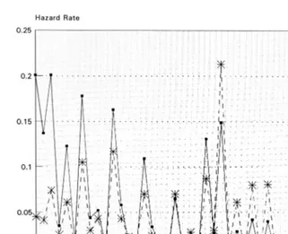
Figs. 1–3 provide some descriptive information on escape rates from unem-ployment and on postunemunem-ployment wage changes of UI recipients and
nonrecipi-Ž .
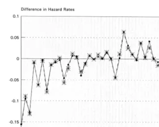
ents from week 2 to week 50 of postdisplacement unemployment . There is clear evidence of a clustering of unemployment spell length observations around monthly intervals in the empirical hazard rates in Fig. 1. There is also a large spike in the hazard rate for UI recipients in the twenty-sixth week, an unemployment duration which corresponds to the maximum eligibility period for unemployment receipt in most jurisdictions. However, the hazard rate is also high at the twenty-sixth week for nonrecipients, suggesting that there may be some rounding in the respondents’ answers to one-half of a year. Fig. 2 graphs the difference in the empirical hazards between recipients and nonrecipients, from which it is clear that the largest difference in hazards between UI recipients and nonrecipients occurs in the twenty-sixth week. It is also clear that escape rates among nonrecipi-ents are much higher than those of recipinonrecipi-ents during weeks 2 through 4, but then gradually come to approach the latter up to the twenty-sixth week. After this point, the hazards of recipients are generally higher than those of nonrecipients. Interest-ingly, there are few signs to suggest that the UI effect is very different for workers suffering shutdowns compared to those who were laid off, even if the latter may have possibly been expecting recall at the start of their displacement.
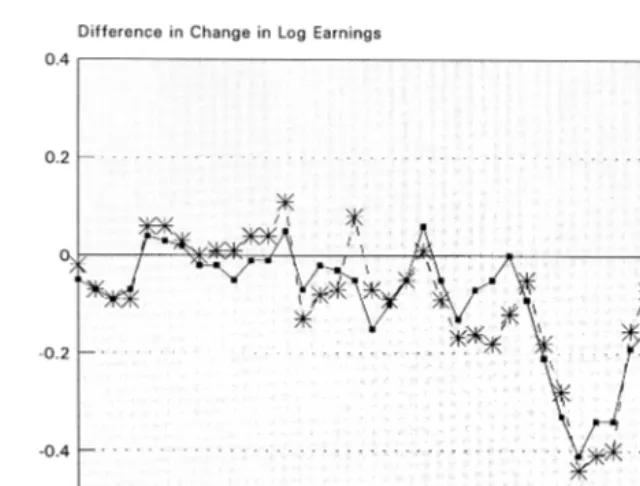
Fig. 3 plots differences between recipient and nonrecipients in the average change in the logarithm of weekly earnings between the current job and the lost job. These average changes are compared for recipients and nonrecipients with the same completed unemployment spell lengths. The major difference between the
16 Ž
Any imputed replacement rates above one because the minimum benefit in the state was greater
.
Fig. 1. Empirical hazard rates by UI receipt.
two groups appears in the 10-week period following the usual exhaustion point for UI benefits. The more rapid job-finding rates among recipients than nonrecipients
Ž .
over this interval see Fig. 2 might thus appear to be associated with a large and rapid decline in their reservation wages. Prior to that interval, there is also some suggestion that recipients on balance have smaller wage gains or larger losses. Once again, there is no clear indication of material differences in the behavior of recipients and nonrecipients by reason for layoff as movements in the wage change gap for shutdowns largely track the overall pattern.
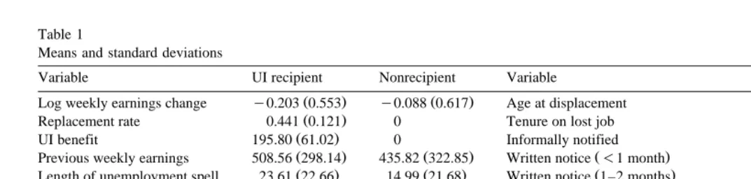
Descriptive statistics for the variables used in our analysis are presented in
Table 1. Separate statistics are presented for UI recipients and nonrecipients.17On
17
Nonrecipients constitute 35% of the combined sample. This is not very different from what one
Ž .
might expect given aggregate unemployment statistics. For example, Burtless 1990 reports that, in October 1985, 37% of the unemployment population consisted of job losers who had been unemployed for less than 6 months. At the same time, 28% of the unemployed population was receiving UI benefits.
Ž
As only job losers are entitled to benefits and extended benefits past 26 weeks were not common in
.
Fig. 2. Difference in hazard rates between recipients and nonrecipients.
average, the change in the logarithm of weekly earnings following displacement is
Ž .
negative for both groups reflecting average wage losses , with the average loss being greater for recipients. The difference between the two groups suggests a wage loss that is on average 11 percentage points higher for recipients than for nonrecipients. The length of the spell of unemployment is also on average about 9 weeks longer for recipients. However, there are other considerable differences between the two groups in variables that might be expected to affect either wage changes or the duration of unemployment. For example, average weekly earnings
on the lost job are more than US$70 higher for recipients.18 As would be
expected, UI recipients tend to have longer tenure on the previous job; they are also more likely to have lost their job as a result of a layoff rather than a plant closing or abolition of position or shift. UI recipients are also more likely to be male, married, blue-collar, older, previously full-time, and a high school graduate. The average estimated replacement rate for UI recipients is 44%, and the average estimated weekly benefit is just under US$200.
18
Ž .
Fig. 3. Difference in log earnings changes between recipients and nonrecipients.
The considerable difference in sample characteristics for recipients and nonre-cipients suggests that controlling for these other factors may be important in assessing the impact of the UI system on subsequent wages. We next estimate regression models for unemployment duration and log wage changes that control for these other influences.
4. Regression model estimates of UI impacts
4.1. Effects using UI recipients only
As noted earlier, virtually all of the previous research into the impact of UI on wages has relied on samples consisting of UI recipients only. Previous studies examining UI and unemployment duration have also tended to use only UI
recipients.19 Most often, these studies use samples derived from official state UI
19 Ž . Ž .
()
J.T.
Addison,
M.L.
Blackburn
r
Labour
Economics
7
2000
21
–
53
Table 1
Means and standard deviations
Variable UI recipient Nonrecipient Variable UI recipient Nonrecipient
Ž . Ž . Ž . Ž .
Log weekly earnings change y0.203 0.553 y0.088 0.617 Age at displacement 35.63 9.91 32.23 10.05
Ž . Ž . Ž .
Replacement rate 0.441 0.121 0 Tenure on lost job 5.57 6.33 3.25 4.82
Ž .
UI benefit 195.80 61.02 0 Informally notified 0.374 0.344
Ž . Ž . Ž .
Previous weekly earnings 508.56 298.14 435.82 322.85 Written notice -1 month 0.061 0.042
Ž . Ž . Ž .
Length of unemployment spell 23.61 22.66 14.99 21.68 Written notice 1–2 months 0.050 0.038
Ž .
Female 0.397 0.436 Written notice )2 months 0.059 0.039
Married 0.652 0.581 High school graduate 0.457 0.372
Black 0.085 0.087 Some college 0.245 0.274
Laid off 0.329 0.254 College graduate 0.169 0.208
Ž . Ž . Ž .
Full-time on lost job 0.962 0.856 Unemployment rate at displacement 6.76 2.14 6.56 2.00
Ž . Ž . Ž .
Blue-collar on lost job 0.482 0.362 Unemployment rate at survey 6.14 1.57 6.10 1.51
rolls, allowing for the collection of exact benefit amounts, but by construction omitting nonrecipients. When using data on UI recipients only, attention has generally focused on the effects of the percentage of earnings replaced by UI and the potential duration of UI benefits. As mentioned in Section 2, we do not have direct reports on UI benefits, but have attempted to estimate benefits using published state-level data.
We first used our sample of UI recipients to estimate reduced-form equations in
Ž .
which the dependent variable is the length of the unemployment spell U :
log U
Ž .
sb1Rqb2Xqe,where R is the replacement rate and X includes the other determinants of unemployment duration detailed in Table 2. We also estimated equations in which the estimated weekly benefit substitutes for the replacement rate. The equations
were estimated by OLS, and the results are presented in Table 2.20
The estimated coefficient for the replacement rate is positive and statistically significant. It suggests that an increase in the replacement rate of 10 percentage points would lead to a 5% increase in the duration of an unemployment spell. The equation that includes the benefit amount as a regressor also suggests that more generous benefits are associated with longer durations, and with a slightly larger effect: an increase in the benefit level of US$50 — roughly 10% of average weekly earnings — leads to an 8% increase in duration. The results also suggest that workers receiving lengthier periods of written notice of their impending job
loss have longer durations than those who do not receive this type of notice.21
Our primary purpose in estimating equations for unemployment duration is to gauge the performance of the imputed benefit variables. If our benefit and replacement rate measures suffered from a substantial degree of measurement error, we would expect that our estimated duration effects would be smaller than those generally reported in the literature that use data with actual unemployment benefits. By this comparison, our results are very encouraging for our imputations. Not only do we find considerable evidence that UI influences unemployment duration, but our estimated effects are also of a similar magnitude to those
Ž .
reported in studies using actual benefits. In particular, Meyer 1990 states that the
20
The unemployment duration equation conforms to an accelerated failure time model. Equations of this type are often estimated by a maximum likelihood procedure that incorporates the inherent
Ž .
censoring of incomplete spells see, for example, Addison and Portugal, 1987 . However, the DWS largely consists of completed spells, with only a small proportion of censored durations at 99 weeks. Given the unimportance of the censoring problem, we prefer to avoid assumptions about the distribution of the error term in the duration equation by using an ordinary least squares estimator. In
Ž
any event, estimations that take into account the censoring of observations with the assumption that
.
unemployment durations are lognormally distributed provided results that are very similar to those reported here.
21
Ž .
()
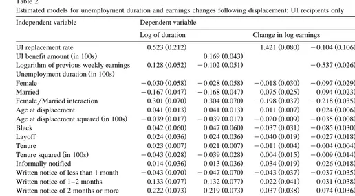
Estimated models for unemployment duration and earnings changes following displacement: UI recipients only Independent variable Dependent variable
Log of duration Change in log earnings
Ž . Ž . Ž . Ž .
UI replacement rate 0.523 0.212 1.421 0.080 y0.104 0.106 y0.072 0.104
Ž . Ž . Ž .
UI benefit amount in 100s 0.169 0.043 0.010 0.021
Ž . Ž . Ž . Ž . Ž .
Logarithm of previous weekly earnings 0.128 0.052 y0.102 0.051 y0.537 0.026 y0.527 0.025 y0.527 0.026
Ž . Ž .
Unemployment duration in 100s y0.416 0.036
Ž . Ž . Ž . Ž . Ž . Ž .
Female y0.030 0.058 y0.028 0.058 y0.018 0.030 y0.097 0.029 y0.097 0.029 y0.094 0.028
Ž . Ž . Ž . Ž . Ž . Ž .
Married y0.167 0.047 y0.168 0.047 0.075 0.025 0.094 0.023 0.095 0.023 0.082 0.023
Ž . Ž . Ž . Ž . Ž . Ž .
FemalerMarried interaction 0.301 0.070 0.304 0.070 y0.198 0.037 y0.218 0.035 y0.218 0.035 y0.192 0.034
Ž . Ž . Ž . Ž . Ž . Ž .
Age at displacement 0.041 0.013 0.041 0.013 0.011 0.007 0.024 0.006 0.024 0.006 0.025 0.006
Ž . Ž . Ž . Ž . Ž . Ž . Ž .
Age at displacement squared in 100s y0.039 0.017 y0.039 0.017 y0.020 0.009 y0.035 0.008 y0.035 0.008 y0.037 0.008
Ž . Ž . Ž . Ž . Ž . Ž .
Black 0.042 0.060 0.047 0.060 y0.037 0.031 y0.085 0.030 y0.084 0.030 y0.082 0.029
Ž . Ž . Ž . Ž . Ž . Ž .
Layoff 0.024 0.036 0.024 0.036 y0.040 0.019 y0.027 0.018 y0.026 0.018 y0.025 0.018
Ž . Ž . Ž . Ž . Ž . Ž .
Tenure 0.023 0.007 0.021 0.007 y0.011 0.004 y0.004 0.004 y0.004 0.004 y0.002 0.004
Ž . Ž . Ž . Ž . Ž . Ž . Ž .
Tenure squared in 100s y0.043 0.028 y0.039 0.028 0.004 0.015 y0.009 0.014 y0.009 0.014 y0.012 0.014
Ž . Ž . Ž . Ž . Ž . Ž .
Informally notified 0.014 0.036 0.013 0.036 0.034 0.019 0.026 0.018 0.027 0.018 0.024 0.018
Ž . Ž . Ž . Ž . Ž . Ž .
Written notice of less than 1 month y0.043 0.070 y0.047 0.070 y0.043 0.037 y0.037 0.035 y0.038 0.035 y0.036 0.034
Ž . Ž . Ž . Ž . Ž . Ž .
Written notice of 1–2 months 0.133 0.077 0.132 0.077 0.022 0.041 0.031 0.038 0.031 0.038 0.041 0.038
Ž . Ž . Ž . Ž . Ž . Ž .
Written notice of 2 months or more 0.222 0.073 0.219 0.073 0.037 0.038 0.074 0.036 0.072 0.036 0.097 0.035
Ž . Ž . Ž . Ž . Ž . Ž .
High school graduate y0.070 0.052 y0.073 0.052 0.045 0.027 0.096 0.026 0.095 0.026 0.086 0.026
Ž . Ž . Ž . Ž . Ž . Ž .
Some college y0.126 0.060 y0.130 0.060 0.026 0.031 0.114 0.030 0.112 0.030 0.100 0.029
Ž . Ž . Ž . Ž . Ž . Ž .
College graduate y0.063 0.069 y0.068 0.069 0.150 0.035 0.287 0.034 0.286 0.034 0.276 0.034
Ž . Ž . Ž . Ž . Ž . Ž .
Full-time worker on previous job 0.021 0.092 0.027 0.091 y0.293 0.046 y0.019 0.046 y0.027 0.045 y0.020 0.045
Ž . Ž . Ž . Ž . Ž . Ž .
Blue-collar worker on previous job 0.051 0.039 0.050 0.039 y0.058 0.020 y0.061 0.019 y0.062 0.019 y0.054 0.019
Ž . Ž . Ž . Ž . Ž . Ž . Ž .
Unemployment rate at displacement 0.056 0.009 0.056 0.009 y0.003 0.006 y0.018 0.006 y0.017 0.006 y0.012 0.006
Ž . Ž . Ž . Ž . Ž .
Unemployment rate at survey y0.020 0.008 0.006 0.007 0.005 0.007 0.006 0.007
2
R 0.066 0.069 0.158 0.248 0.248 0.275
typical estimate of the UI effect suggests that a 10% increase in the UI
replace-Ž
ment rate increases the duration of unemployment spells by about 1 week his own
.
results suggest an increase of one-and-a-half weeks . Our two estimates suggest that a 10% increase in benefits would increase unemployment by one to
one-and-Ž .
a-half weeks at the average unemployment duration of 24 weeks .
We are of course primarily interested in the wage effects of UI. The dependent variable in our wage equations is the difference between the log of weekly
Ž .
earnings at the time of the survey Ws and the log of weekly earnings on the lost
Ž .
job W :p
log W
Ž
srWp.
sg1Rqg2Xqu.Estimates of these regressions are presented in the last four columns of Table 2. One issue in our choice of independent variables is whether the log of previous weekly earnings should be included as a regressor. If there is measurement error in weekly earnings, then a negative and possibly significant coefficient estimate on
lagged earnings may arise when the true coefficient is zero.22 On the other hand,
if there is any tendency for a regression-to-the-mean phenomenon in earnings as a result of displacement, then the coefficient on previous earnings should be negative. This decision is clearly of importance to the estimate of the UI effect, as can be seen by comparing the third and fourth columns of Table 2. If previous
Ž .
earnings are omitted as in the third column , the replacement rate has a large and statistically significant positive effect on the change in log wages. But the replacement rate is negatively correlated with previous earnings, so that once
Ž .
previous earnings are included in the regression as in the fourth column , the coefficient estimate for the replacement rate is negative and statistically insignifi-cant. There is also little evidence that the weekly benefit amount affects the wage change, once previous earnings are controlled for in the regression. In both of these cases, the previous earnings variable is statistically significant. Our own sense is that it is more important to allow for the possibility that there are influences on the wage for the previous job that may not carry over to the wage
Ž .
for the new job such as specific human capital , so that the results that include previous earnings as a regressor are more appropriate.
22
Including previous earnings as an independent variable in a wage change regression is equivalent to regressing the log of survey earnings on the log of previous earnings. Coefficient estimates and standard errors for all variables except the previous earnings variables will be identical under either specification. The coefficient on previous earnings in the wage change equation can be interpreted as a measure of the extent to which earnings levels carry over from the previous job to the new job. A value of zero for that coefficient implies there is complete carryover; a value ofy1 implies there is no carry over. Measurement error in previous earnings would lead to a negative bias in the coefficient estimate
Ž
in our specification because the same measurement error term would appear in both the dependent and
.
There may also be a concern that the replacement rate coefficient is biased because of a nonlinear relationship between the change in log wages and the log of
Ž
previous earnings given that the replacement rate is a function of previous
.
earnings . To consider this possibility, we added additional powers of the log of
Ž .
previous earnings as regressors up to the fifth power . Allowing for this change in specification had no material effects on the coefficient estimates and associated inference.
We believe it is important to control for state-level business cycle conditions that might influence wages, since the state of the economy might be related to the level of UI benefits. However, given that our postunemployment wage is observed
Ž .
at the time of the survey which may be a few years since the displacement event , economic conditions both at the time of the displacement and at the time of the survey could have affected the postunemployment wage. Therefore, we included unemployment rates at both points in time as independent variables in our wage-change equations. Inclusion of these business-cycle controls had only very small effects on the estimated UI impact on wages. It is also interesting to note that, once previous earnings are included as a regressor, of the two, it is the unemployment rate around the time of the initial job search that appears to be more important to the postunemployment wage.
The estimated UI effects do not accord with the previous findings of Burgess
Ž .
and Kingston 1976 that there are significant effects on wages. One difference in our estimation strategies is that Burgess and Kingston include unemployment duration as a regressor in their wage change equations. Duration and postunem-ployment wages would seem to be clearly simultaneously determined, in the standard search model, as they are both functions of the choice of reservation wage. Thus, we prefer a reduced-form strategy that would exclude duration from
the wage change equation.23 To consider the importance of this choice of
specification to our findings, however, we also estimated wage change models that
Ž .
add unemployment duration as a regressor see the final column of Table 2 . This addition proved immaterial to the measure of the UI effects. It would appear that the differences in our findings relate more to the nature of our samples than to
specification issues or UI measures.24
23
One possibility would be to include unemployment duration as a regressor and estimate using instrumental variables. However, it is not obvious that suitable instruments are available for our data. Identification of this effect is made problematic by the fact that both the wage change and duration are functions of the reservation wage, so that any variable that affects one should affect the other. In any
Ž .
case, our goal is to estimate the effect of a change in an exogenous variable UI benefits on the
Ž .
eventual value of an endogenous variable the wage change , which is supplied by the reduced-form coefficient estimate.
24 Ž .
This is perhaps to be expected given that Holen 1977 found results similar to Burgess and
Ž .
We also examined whether the evidence points to stronger UI effects among certain subgroups of the population. For example, it might be that UI increases the benefits of search most for individuals with stronger ties to the labor market, such as men compared with women. UI effects might also be expected to be stronger for workers who have no expectations of being recalled to their employers, that is,
those workers displaced because of a plant closing.25 We also considered whether
Ž
UI effects are stronger for older workers as suggested by the results of Ehrenberg
.
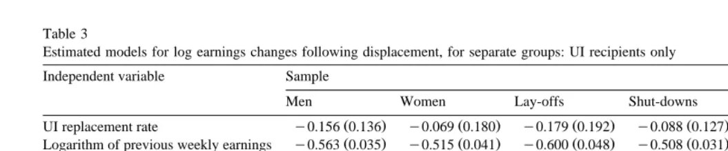
and Oaxaca, 1976 . Accordingly, Table 3 reports estimates of separate wage change models for males and females, for layoffs and shutdowns, and for those below or above age 30, using the replacement rate as the UI variable. In every case, the data suggest that the wage change models do vary across the particular sample bifurcation. By the same token, there is little evidence that the UI effects are different, and in none of the cases is the estimated UI effect positive.
Perhaps the most interesting difference across groups is that lengthier periods of written notice appear to affect wage changes for some groups, but not for others. Our earlier results in Table 2 provided some broad indication that wage changes might be higher for workers in receipt of 2 or more months’ notice of their impending displacement. When the sample is disaggregated, this effect is most strongly supported for the subsamples of women and those displaced by
shut-Ž
downs. This latter finding is quite sensible notified workers who are laid off, but
.
expect recall may not use the notice interval for productive new-job search , but we have no explanation for why notice ‘works’ in this sense for women, but not
for men.26
Our estimates in this section have represented an attempt to replicate the kind
Ž . Ž .
of approach used by Burgess and Kingston 1976 , Holen 1977 , and Classen
Ž1977 . Our results tend to support the conclusions of Classen that more generous.
UI benefits are not associated with larger or smaller wage changes. However, these estimates ignore the potential information on UI effects in the wage changes of nonrecipients. In Sections 4.2 and 4.3, we consider two different methods for incorporating this information in the analysis.
4.2. UI dummyÕariable effects
The simplest way to assess the effects of the UI system would be to compare the average postunemployment outcomes of recipients and nonrecipients. This is
25
We group workers displaced because of an abolition of shift or position with those displaced by plant closings, as they are also unlikely to expect recall to the previous employer. None of the workers in the layoff subsample were actually recalled to their employer, but it is still possible that many of these workers may have begun their unemployment spell anticipating recall.
26 Ž .
()
J.T.
Addison,
M.L.
Blackburn
r
Labour
Economics
7
2000
21
–
53
Table 3
Estimated models for log earnings changes following displacement, for separate groups: UI recipients only
Independent variable Sample
Men Women Lay-offs Shut-downs Age under 30 Age 30 or over
Ž . Ž . Ž . Ž . Ž . Ž .
UI replacement rate y0.156 0.136 y0.069 0.180 y0.179 0.192 y0.088 0.127 y0.110 0.183 y0.044 0.131
Ž . Ž . Ž . Ž . Ž . Ž .
Logarithm of previous weekly earnings y0.563 0.035 y0.515 0.041 y0.600 0.048 y0.508 0.031 y0.618 0.043 y0.492 0.033
Ž . Ž . Ž . Ž . Ž . Ž .
Informal notice 0.026 0.022 0.029 0.032 0.062 0.032 0.011 0.022 y0.022 0.031 0.046 0.022
Ž . Ž . Ž . Ž . Ž . Ž .
Written notice of less than 1 month y0.017 0.043 y0.065 0.059 y0.073 0.056 y0.007 0.045 y0.080 0.059 y0.014 0.043
Ž . Ž . Ž . Ž . Ž . Ž .
Written notice of 2 months or more y0.009 0.048 0.140 0.056 y0.049 0.101 0.090 0.039 0.053 0.073 0.078 0.042 P-value of test for equal coefficients 0.000 0.000 0.000 0.000 0.000 0.000
n 2149 1414 1172 2391 1143 2420
2
R 0.285 0.214 0.249 0.242 0.303 0.221
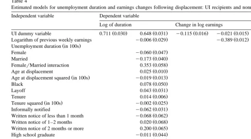
in essence what we did in constructing Figs. 2 and 3, discussed earlier. Of course, these comparisons are only informative if recipients and nonrecipients do not differ along any other dimensions that might be expected to affect search outcomes. As this is unlikely to be the case, we now extend this type of comparison by using a sample of recipients and nonrecipients to estimate equa-tions for unemployment outcomes that include a UI dummy variable along with
other wage determinants as independent variables.27 Estimated models in which
either the log of unemployment duration or the change in the log of earnings is the dependent variable are reported in Table 4.
As a preliminary to this analysis, two very simple models — with the UI dummy as the only regressor — were estimated. They indicate that UI recipients have statistically significantly longer unemployment spells, and have wage changes that are on average less then those of nonrecipients. The effect of UI receipt on the duration of the unemployment spell is virtually unaffected by the inclusion of other control variables in the model, the coefficient falling from 0.71 to 0.65 and remaining highly statistically significant. When the same set of controls are added to the wage change equation, however, the UI coefficient estimate changes sign
and loses any clear statistical significance in a test that the coefficient is zero.28
This is largely the result of including previous earnings as a control, as can be seen from the change in the estimated UI coefficient when only the previous earnings variable is included as an additional control. The effect of UI is positive, larger, and statistically significant when unemployment duration is included as a regressor
Žas in Burgess and Kingston, 1976 , but as was argued earlier, this is not likely to.
be an appropriate strategy for estimating UI effects on wage changes.
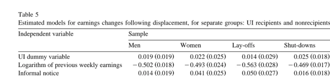
We again estimated separate models according to sex, type of displacement, and age. These results are reported in Table 5. All coefficient estimates are positive, and there is little statistical evidence that the UI effects vary across the groups. The coefficient estimate is higher for shutdowns than for layoffs, as we would expect, but the difference is not statistically significant. The estimated notice effects on wage changes are smaller once we include UI nonrecipients in
Ž .
the sample compare Table 3 , although they still provide the suggestion that women, workers who lost jobs through shutdowns, and older individuals gain more from the notice interval.
27
This approach will control for observable differences only. In an attempt to ascertain whether UI
Ž .
effects were robust to unobservable differences and to measurement error in the UI variable , we estimated our wage equations instrumenting for the UI dummy variable, where our instruments are the state-level parameters of the UI program used earlier to construct replacement rates for the UI recipient sample. However, the low degree of correlation between these parameters and the UI dummy caused a considerable increase in the standard error of the UI dummy variable coefficient estimate, suggesting that OLS estimates may be preferable to these IV estimates.
28
()
Estimated models for unemployment duration and earnings changes following displacement: UI recipients and nonrecipients Independent variable Dependent variable
Log of duration Change in log earnings
Ž . Ž . Ž . Ž . Ž . Ž .
UI dummy variable 0.711 0.030 0.648 0.031 y0.115 0.016 y0.021 0.015 0.021 0.015 0.049 0.015
Ž . Ž . Ž . Ž .
Logarithm of previous weekly earnings y0.006 0.029 y0.389 0.012 y0.496 0.014 y0.495 0.014
Ž . Ž .
Unemployment duration in 100s y0.391 0.031
Ž . Ž . Ž .
Female y0.060 0.047 y0.070 0.023 y0.071 0.023
Ž . Ž . Ž .
Married y0.173 0.040 0.122 0.019 0.112 0.019
Ž . Ž . Ž .
FemalerMarried interaction 0.353 0.058 y0.236 0.029 y0.208 0.028
Ž . Ž . Ž .
Age at displacement 0.025 0.010 0.026 0.005 0.027 0.005
Ž . Ž . Ž . Ž .
Age at displacement squared in 100s y0.019 0.013 y0.039 0.007 y0.039 0.007
Ž . Ž . Ž .
Black 0.078 0.050 y0.048 0.025 y0.040 0.024
Ž . Ž . Ž .
Layoff 0.043 0.031 y0.020 0.015 y0.017 0.015
Ž . Ž . Ž .
Tenure 0.014 0.006 y0.002 0.003 y0.001 0.003
Ž . Ž . Ž . Ž .
Tenure squared in 100s y0.002 0.025 y0.014 0.012 y0.014 0.012
Ž . Ž . Ž .
Informally notified y0.062 0.031 0.023 0.015 0.018 0.015
Ž . Ž . Ž .
Written notice of less than 1 month y0.068 0.062 y0.028 0.031 y0.030 0.030
Ž . Ž . Ž .
Written notice of 1–2 months 0.020 0.068 0.021 0.033 0.026 0.033
Ž . Ž . Ž .
Written notice of 2 months or more 0.200 0.065 0.050 0.032 0.066 0.031
Ž . Ž . Ž .
High school graduate y0.011 0.044 0.101 0.022 0.097 0.021
Ž . Ž . Ž .
Some college y0.111 0.049 0.120 0.024 0.107 0.024
Ž . Ž . Ž .
College graduate y0.027 0.056 0.318 0.027 0.311 0.027
Ž . Ž . Ž .
Full-time worker on previous job y0.229 0.060 y0.025 0.029 y0.041 0.029
Ž . Ž . Ž .
Blue-collar worker on previous job 0.023 0.033 y0.049 0.016 y0.044 0.016
Ž . Ž . Ž . Ž .
Unemployment rate at displacement 0.052 0.008 y0.013 0.005 y0.009 0.005
Ž . Ž . Ž .
Unemployment rate at survey y0.003 0.006 y0.002 0.006
Other controls No Yes No No Yes Yes
2
R 0.096 0.145 0.009 0.178 0.260 0.282
()
Addison,
M.L.
Blackburn
r
Labour
Economics
7
2000
21
–
53
43
Table 5
Estimated models for earnings changes following displacement, for separate groups: UI recipients and nonrecipients
Independent variable Sample
Men Women Lay-offs Shut-downs Age under 30 Age 30 or over
Ž . Ž . Ž . Ž . Ž . Ž .
UI dummy variable 0.019 0.019 0.022 0.025 0.014 0.029 0.025 0.018 0.033 0.024 0.015 0.019
Ž . Ž . Ž . Ž . Ž . Ž .
Logarithm of previous weekly earnings y0.502 0.018 y0.493 0.024 y0.563 0.028 y0.469 0.017 y0.557 0.024 y0.464 0.018
Ž . Ž . Ž . Ž . Ž . Ž .
Informal notice 0.014 0.019 0.041 0.025 0.050 0.027 0.016 0.018 y0.002 0.024 0.035 0.019
Ž . Ž . Ž . Ž . Ž . Ž .
Written notice of less than 1 month y0.041 0.039 y0.006 0.050 y0.082 0.050 0.006 0.039 y0.008 0.051 y0.042 0.038
Ž . Ž . Ž . Ž . Ž . Ž .
Written notice of 1–2 months 0.076 0.044 y0.031 0.052 y0.181 0.082 0.064 0.037 y0.031 0.057 0.045 0.041
Ž . Ž . Ž . Ž . Ž . Ž .
Written notice of 2 months or more y0.020 0.043 0.115 0.048 y0.107 0.092 0.070 0.034 0.033 0.061 0.056 0.037 P-value of test for equal coefficients 0.000 0.000 0.000 0.000 0.000 0.000
n 3227 2247 1658 3816 2039 3435
2
R 0.270 0.256 0.275 0.262 0.299 0.225
It is somewhat problematic to ascertain the nature of the support that our estimates provide for the existence of a UI effect on wage changes. The UI dummy variable coefficient estimate could be called marginally significant in a one-sided test, but then only at a significance level greater than 0.081. Yet the point estimate would represent a fairly sizeable effect — a 2% increase for a worker with weekly earnings of US$400 would imply an extra US$412 dollars per year. If this effect were to persist, then at a 10% discount rate it would have a present value of roughly US$4000. Of course, many of the earlier studies suggested an even larger expected effect of the UI system. For example, Burgess and Kingston’s results suggest that a change in the weekly UI benefit from zero
Žfor a nonrecipient to the sample average should increase earnings by 45%, while.
Holen’s results suggest a 64% increase.29 Blau and Robin’s results would suggest
about a 5% increase in earnings from a change in the replacement rate from 0 to 45%, although this estimated effect is not statistically significant. Ehrenberg and Oaxaca’s results would point to a 9% increase in earnings for a similar comparison using their results for older males. Ehrenberg and Oaxaca’s results only
approxi-mate ours when they predict a 3% increase for older women.30
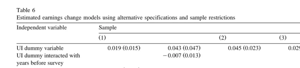
We also explored the robustness of the estimated UI effect on wage changes to the specification of tenure effects. Because nonrecipients tend to have low levels of tenure, we added to our specification two dummy variables signifying that the recipient had zero years or 1 year of tenure with their previous employer. These
Ž .
results presented in the first column of Table 6 show that the estimated effects are not sensitive to the inclusion of these dummies. We also tried adding additional powers of tenure to our base specification. Although these additional powers for tenure proved to be statistically significant through the fourth power, their inclusion did not affect the estimated impact of UI. The addition of higher powers for the log of previous earnings to our specification also proved inconse-quential to the estimated UI effect.
We looked for evidence of the persistence of UI effects by interacting the UI dummy with the number of years between the displacement event and the survey date at which the earnings information was collected. If there is a positive effect that dissipates over time, then we should expect a large UI dummy effect and a
29
Holen does not present average benefits or earnings for her sample, so we combined the averages from Burgess and Kingston with the coefficient estimates from Holen.
30
Ehrenberg and Oaxaca’s point estimates for younger men and women would suggest that UI recipients receive a 5% wage advantage among young men and a 2% wage advantage among young
Ž .
women assuming an average UI replacement rate of 0.50 . Classen does not provide means, but using
Ž .
Burgess and Kingston’s average benefits and earnings from a time period similar to Classen’s
Ž
suggests that UI recipients receive either a 3% postunemployment wage advantage using her
. Ž .
negative coefficient on the interaction variable. This is indeed the pattern that the
Ž .
coefficient estimates reflect see the second column of Table 6 , but the interaction
coefficient estimate is not statistically significant.31
Our ideal measure of UI status would be an indicator of the UI eligibility of displaced workers, but the information from the DWS only identifies recipiency status. There may have been many workers who were eligible for UI, and who were unemployed for more than a week, but who chose not to apply for UI benefits. We were also concerned that there may be some measurement error in the report of recipiency status. In an attempt to construct a measure that may be more closely related to eligibility status, we combined information on receipt of UI with information on tenure. Given that workers are largely eligible for UI if they are displaced and have at least 1 year of tenure on the lost job, we excluded from
Ž
our sample all nonrecipients with reported tenure of more than 1 year. We also excluded all UI recipients who reported zero years of tenure with the old
.
employer. Results using this alternative sample are reported in the column using
Ž .
sample 2 in Table 6, and provide perhaps our strongest evidence in favor of an wage-increasing effect of UI; the coefficient estimate is larger than before and is now clearly statistically significant. This support is undermined by the fact that the redefined sample makes the UI dummy variable much more highly correlated with tenure, so that it is impossible to separately identify the UI effect and any deviations of the tenure profile from the quadratic specification that might occur at very low levels of tenure.
Using our original UI recipiency variable, we estimated two additional models to check the importance of the restrictions in our sample definition to the estimates of the model. First, we removed the restriction that the displacement had to occur at least 1 year before the survey. As discussed in Section 2, this restriction was imposed to avoid a possible selection of workers on the basis of how long they
Ž .
stayed unemployed. Its removal see the penultimate column of Table 6 causes a slight increase in the estimated coefficient on the UI dummy, so that the restriction
Ž
does not appear to be very consequential although the fall in the standard error
.
leaves the estimate statistically significant at the 5% level . More important is the qualification that the unemployment spell lasts at least 2 weeks. This would seem to be an important restriction in evaluating the importance of access to UI on subsequent wage changes, because many of the UI nonrecipients with durations less than 2 weeks may have actually been eligible for UI benefits. After this
Ž .
restriction is removed the last column of Table 6 , the UI coefficient estimate becomes negative and statistically significant, suggesting that the receipt of UI
31
()
J.T.
Addison,
M.L.
Blackburn
r
Labour
Economics
7
2000
21
–
53
Table 6
Estimated earnings change models using alternative specifications and sample restrictions Independent variable Sample
Ž .1 Ž .2 Ž .3 Ž .4
Ž . Ž . Ž . Ž . Ž .
UI dummy variable 0.019 0.015 0.043 0.047 0.045 0.023 0.029 0.013 y0.030 0.013
Ž .
UI dummy interacted with y0.007 0.013
years before survey
Ž .
Dummy for tenures0 y0.034 0.025
Ž .
Dummy for tenures1 y0.018 0.022
Ž . Ž . Ž . Ž . Ž .
Tenure y0.005 0.004 y0.002 0.003 y0.006 0.004 y0.002 0.003 0.002 0.003
Ž . Ž . Ž . Ž . Ž . Ž .
Tenure squared in 100s y0.004 0.014 y0.014 0.012 0.002 0.015 y0.015 0.011 y0.027 0.011
n 5474 5474 4072 6984 6917
2
R 0.261 0.260 0.248 0.235 0.262
Notes: The dependent variable is the change in log earnings. All specifications included the same set of additional controls as in the fifth column of Table 4.
Ž . Ž . Ž .
The samples are defined as follows: sample 1 is the same as that used in estimating the equations reported in Table 4; sample 2 drops from sample 1 all
Ž .
observations that report being nonrecipients and having more than 1 year of tenure, or report being recipients with tenure of less than 1 year; sample 3 adds
Ž . Ž . Ž . Ž .
to sample 1 all observations that were displaced within 1 year of the survey but were unemployed for at least 2 weeks ; and, sample 4 adds to sample 1
Ž .
benefits lowers the size of the wage change following unemployment. In abandon-ing this restriction, however, we are classifyabandon-ing many individuals as nonrecipients only because they were able to find a job — presumably because of a good wage
draw — before their eligibility for UI benefits began.32
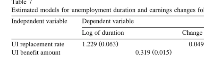
4.3. UI replacement rate effects including the nonrecipient sample
Ž .
As noted earlier, both Ehrenberg and Oaxaca 1976 and Blau and Robins
Ž1986 also include nonrecipients in their sample, but used the replacement rate as.
Ž .
their UI-related variable treating the replacement rate of nonrecipients as zero . Table 7 provides the results of a parallel analysis using our data. In these results, UI has an even larger estimated effect on unemployment duration than was the
Ž .
case when nonrecipients were excluded Table 2 , whether we use replacement
Ž .
rates or benefits treating the nonrecipient benefit as zero . In the wage change equation, however, the estimated effect of the replacement rate is positive, but as with the UI dummy variable, only weakly significant. The magnitude of the coefficient estimate suggests a similar effect to that using the UI dummy variable
Ž .
— going from a rate of zero to one of 0.44 the average for UI recipients is
predicted to increase subsequent earnings by about 2%.33 The coefficient estimate
is even less supportive of a UI effect when we use UI benefit amounts rather than replacement rates. On the whole, it would seem that this alternative specification of the UI indicator provides conclusions similar to the dummy variable specifica-tions.
We also estimated models that defined the replacement rate for nonrecipients differently from that used for the Table 7 estimates. Instead of using the actual replacement rate of zero, we used the replacement rate associated with the benefit they would have received if they had taken up UI. This follows a suggestion of
Ž .
Portugal and Addison 1990 , and effectively makes the replacement rate variable
Ž
exogenous to UI receipt. This model can be interpreted as a reduced form of the dummy variable model, in which UI receipt is modelled as a linear function of the
.
potential replacement rate for each individual . For this estimation, we also removed the restriction that the unemployment spell be of at least 2 weeks in
32
We also re-estimated our wage change equation after increasing the number of weeks of unemployment necessary to be included in the sample. If we use only observations with unemployment spells of 3 weeks or more, the coefficient estimate increases and is clearly statistically significant. As we continue to increase the cutoff point for sample inclusion, the coefficient estimate tends be in the
Ž
range of 7–8% and statistically significant until it begins to fall again after 30 or so weeks of
.
unemployment . To the extent that support for a UI effect on wages can be adduced from our results, this conclusion is sensitive mainly to the exclusion of individuals with spells of unemployment lasting less than 2 weeks.
33
Using this specification of the UI variable, Ehrenberg and Oaxaca find strong evidence of a positive UI coefficient for older individuals. We also estimated our model for separate age groups
Table 7
Estimated models for unemployment duration and earnings changes following displacement Independent variable Dependent variable
Log of duration Change in log earnings
Ž . Ž .
UI replacement rate 1.229 0.063 0.049 0.031
Ž . Ž .
UI benefit amount 0.319 0.015 0.007 0.007
Žin 100s of dollars.
Ž . Ž . Ž . Ž .
Logarithm of previous 0.128 0.030 y0.136 0.030 y0.491 0.015 y0.498 0.015 weekly earnings
2
R 0.136 0.147 0.260 0.260
Notes: Numbers in parentheses are standard errors. The sample size is 5474. All specifications include the other controls used in the first and fourth columns of Table 2.
duration. Given that the results were quite sensitive to the specification for the log of the previous earnings variables, we also included several powers of this variable as independent variables. Once we did so, the replacement rate coefficient was essentially the same as in Table 7, with a much larger standard error.
4.4. UI and subsequent job stability
If UI allows workers to search longer before taking a job, then one possible beneficial effect of UI might be that workers can take more desirable jobs which they will be less likely to quit. This may be because they take jobs that represent better matches between employer and worker. If there is such an effect, then we should expect to see less subsequent job changing after finding a new job for UI recipients than for nonrecipients. The DWS provides an indicator of the number of jobs that the worker has held since the displacement event. We used this indicator to explore whether UI recipients had a more stable work history following displacement than nonrecipients.
To test this effect, we estimated logistic regression models for the probability
Ž
that the respondent held only one job following displacement rather than holding
.
more than one job . In these specifications, we included the same set of additional
controls as in our earlier models for unemployment duration and wage changes.34
The results are reported in Table 8. The coefficient estimate for the UI dummy is positive — suggesting that UI recipients are more likely to have held only one job — but its t-statistic is only 1.04. Its magnitude is also fairly small, translating into an increase of only about 1 percentage point in the probability of holding just one
34