The labor market effects of non-wage
compensations
Masanori Hashimoto
), Jingang Zhao
Department of Economics, The Ohio State UniÕersity, 1945 North High Street, Columbus,
OH 43210-1172, USA
Received 1 June 1997; accepted 1 February 1999
Abstract
Contrary to the argument that non-wage compensation is a tax on labor reducing employment, we find that employment may increase in response to an increased demand for
Ž
benefits a decreased cost of providing benefits or increased government-mandated benefit .
levels , under the assumption of strong cross-economies of scale. When there are strong cross-diseconomies of scale, employment and hours both decrease. The secular increase in employer-provided insurance and the growth in U.S. employment may well reflect the role of cross-economies of scale, which seems to exist in larger firms with lower marginal non-wage benefit costs.q2000 Elsevier Science B.V. All rights reserved.
JEL classification: J30; J32; J38
Keywords: Employment; Fringe benefits; Labor market; Non-wage compensation
1. Introduction
Non-wage compensation measured as a percentage of total labor compensation has risen significantly in the United States and other developed countries over the
Ž .
past few decades Hart et al., 1988 . For example, in the firms surveyed by the
)
Corresponding author. Tel.: q1-614-292-4196; fax: q1-614-292-3906. E-mail addresses:
Ž . Ž .
[email protected] M. Hashimoto ; [email protected] J. Zhao
0927-5371r00r$ - see front matterq2000 Elsevier Science B.V. All rights reserved.
Ž .
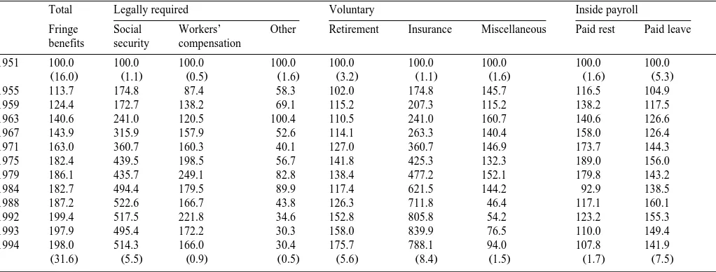
Chamber of Commerce, fringe benefits grew from 16.0% of total compensation in
Ž .
1951 to 31.6% in 1994 see Table 1 . Two fringe benefit items have experienced particularly large increases over this period: Social Security has increased from 1.1
Ž
to 5.5% of total compensation, while the insurance component life, health, and
. 1
dental premiums; death benefits has risen from 1.1 to 8.4%. Existing economic analyses suggest that, to the extent that these non-wage payments are quasi-fixed costs, such increases in fringe benefits should reduce employment.2 The argument is that non-wage compensation is a tax on labor that increases total labor cost inducing employers to reduce employment.
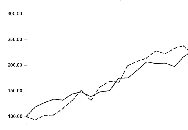
Because they have been conducted at the firm level, previous analyses tend to assume non-wage payments to be exogenous.3As Fig. 1 demonstrates, both the
Ž . Ž .
legally required exogenous and the voluntary endogenous components of fringe benefits have grown substantially over the past 40 years, with the voluntary component far outpacing the legally required component after the early 1980s. Clearly, a comprehensive analysis would require that non-wage compensation be modeled as endogenous since the voluntary increases in these payments surely are induced by the market.
Accordingly, we present a market level analysis to see how an increase in non-wage benefits affects equilibrium employment, wages, and benefit levels. We focus on three exogenous sources of increased benefits; an increase in the demand for benefits, a decrease in the cost of providing benefits, and an increase in the mandated benefits. Contrary to the conventional view, our analysis shows that employment may increase, rather than decrease, in response to increased non-wage payments.
Our predictions depend critically on whether there exist cross-scale effects.
Ž .
There exist cross-economies of scale if an increase in benefits employment
Ž .
lowers the marginal non-wage cost of employment benefits . The opposite case exhibits cross-diseconomies of scale.
Our main findings are as follows. When there are strong cross-economies of scale, employment and benefits rise and hours of work and the wage fall. When
1
Ž . Ž
The U.S. Bureau of Labor Statistics BLS United States Department of Labor, Bureau of Labor
.
Statistics, 1977, 1995 is another source of benefit data, but its data is available only for the years 1966–1974 and 1987–1995. The available BLS data show similar trends in the growth of the components of fringe benefits. For example, social security climbed from 3.2 to 6.0% of total compensation from 1966 to 1995; insurance rose from 2.0 to 6.7% over the same period. Overall,
w
fringe benefits grew from 16.9 to 28.3% of total compensation. See Hashimoto, 1994 for an update in
x
Table 1 of Woodbury, 1983. 2
This analytical result seems robust to various assumptions. In particular, when the model of employment-hours decisions is expanded to allow for changes in capital, many of the results concerning hours become ambiguous; however, the fixed-cost effect on employment remains intact
ŽHart, 1984; Hamermesh, 1993 ..
3 Ž . Ž . Ž . Ž .
See, for example, Oi 1962 , Rosen 1968 , Ehrenberg 1971 , Hart 1984 , and Hamermesh
()
M.
Hashimoto,
J.
Zhao
r
Labour
Economics
7
2000
55
–
78
57
.
United States, 1981
The numbers in parentheses are the percentage of fringe benefits in total compensation.
Legally required benefits are contributions to social security, federal and state unemployment insurance, and workers’ compensation.
Ž .
Benefits provided voluntarily by the employer include private insurance life, health, and accidental , privately sponsored retirement and savings plans
Žpensions, savings and thrift plans , as well as other items severance pay, supplemental unemployment benefits, and other miscellaneous benefits .. Ž . Ž
Source: authors’ calculation based on the data from U.S. Chamber of Commerce, Employee Benefits, various years Chamber of Commerce of the United
.
States, 1985, 1989, 1993, 1994, 1995 .
Total Legally required Voluntary Inside payroll
Fringe Social Workers’ Other Retirement Insurance Miscellaneous Paid rest Paid leave
benefits security compensation
1951 100.0 100.0 100.0 100.0 100.0 100.0 100.0 100.0 100.0
Ž16.0. Ž1.1. Ž0.5. Ž1.6. Ž3.2. Ž1.1. Ž1.6. Ž1.6. Ž5.3.
1955 113.7 174.8 87.4 58.3 102.0 174.8 145.7 116.5 104.9
1959 124.4 172.7 138.2 69.1 115.2 207.3 115.2 138.2 117.5
1963 140.6 241.0 120.5 100.4 110.5 241.0 160.7 140.6 126.6
1967 143.9 315.9 157.9 52.6 114.1 263.3 140.4 158.0 126.4
1971 163.0 360.7 160.3 40.1 127.0 360.7 146.9 173.7 144.3
1975 182.4 439.5 198.5 56.7 141.8 425.3 132.3 189.0 156.0
1979 186.1 435.7 249.1 82.8 138.4 477.2 152.1 179.8 143.2
1984 182.7 494.4 179.5 89.9 117.4 621.5 144.2 92.9 138.5
1988 187.2 522.6 166.7 43.8 126.3 711.8 46.4 117.1 160.1
1992 199.4 517.5 221.8 34.6 152.8 805.8 54.2 123.2 155.3
1993 197.9 495.4 172.2 30.3 158.0 839.9 76.5 110.0 149.4
1994 198.0 514.3 166.0 30.4 175.7 788.1 94.0 107.8 141.9
[image:3.842.86.597.164.358.2]Ž
Fig. 1. Fringe benefits of workers in firms surveyed by the chamber of commerce indices of benefits
.
as a percent of total compensation, 1951s100 .
there are strong cross-diseconomies of scale, however, employment and hours both fall, but the effects on benefits and wage are ambiguous. It is worth noting that, under reasonable assumptions about cross-economies, an increase in fringe bene-fits can raise equilibrium employment. Note that, at least in the United States, insurance has emerged as not only the fastest growing component of fringe benefits but also the largest. It is possible that increases in insurance and other benefits may have contributed to the growth of U.S. employment during the past several decades.
2. Description of the problem
We conduct the analysis using the social welfare maximization problem, where social welfare refers to the sum of the employer and employee surpluses. Suppose the inverse demand and supply functions of labor are, respectively,
WdsWd
Ž .
EŽ
sf E;h,GŽ
.
.
,Ž .
1WssWs
Ž .
EŽ
sg E;h,GŽ
.
.
.Ž .
2These functions are parameterized by standard hours, h, and non-wage benefits, G. Social welfare is given by
E d s
where E is the equilibrium level of employment. Market forces drive social welfare to its maximum,
<
max Z E, h,G E, h,G
Ž
.
G0 ,4
Ž .
4satisfying the first order conditions:
EZrEEs0, EErEhs0, EErEGs0.
Ž .
5Ž
One may analyze the effects of exogenous changes such as an increase in
.
worker demand for benefits by totally differentiating the equations summarized
Ž .
by Eq. 5 . In order to conduct such analysis, the second order condition, that the
Ž .
Hessian matrix of Z E, h,G be negative definite, must hold. Rather than arbitrar-ily imposing this key condition, we derive the market labor demand from the individual firm’s profit-maximization problem in such a way as to be consistent with the second order condition. In fact, our formulation of the firm’s profit-maxi-mization problem leads to the simplest possible functional form for the market labor demand supporting the second order condition.4
2.1. Firm’s decision
Assume that a competitive industry consists of identical firms and that a firm’s labor expenses consist of both wage and non-wage costs as follows:
usu
Ž
n, h,G.
swhnqC G, n n,Ž
.
Ž .
6where n is employment, h is hours of work per worker, G is the quantity of fringe benefits per worker, and w is the hourly wage rate.5 We assume the non-wage cost function, C, to satisfy the following conditions:
C1)0, C11)0, C2,0, C22s0, C12sC21,0.
We call C the marginal non-wage cost of benefits, and C the marginal non-wage1 2 cost of employment. We specify the marginal non-wage cost of benefits to be
Ž . Ž .
positive C1)0 and rising C11)0 . For simplicity, the marginal non-wage cost
Ž .
of employment is assumed be a constant C22s0 , which may be any real number
ŽC2,0 ..
Ž .
The expression C12 sC21 represents cross-scale effects. If C12-0, an
Ž . Ž .
increase in benefits G lowers the marginal non-wage cost of employment C .2 Ž .
Symmetrically, an increase in employment n lowers the marginal non-wage cost
4
Note that the market labor demand and supply functions cannot both be linear. If this were the case, the Hessian matrix for the social welfare function, Z, would not be negative definite. Under the simplification of linear labor supply, the simplest demand form is quadratic.
5
We assume for simplicity that non-wage labor costs are quasi-fixed, or that they are independent of hours of work. Although some non-wage labor costs do depend upon hours of work, approximately
Ž .
Ž .
of benefits C . We define these phenomena as cross-economies of scale. In1 contrast, the case of C12)0 represents cross-diseconomies of scale.
We argue that cross-economies are empirically plausible, since larger firms are likely to have lower marginal non-wage cost of benefits for the following reasons. First, larger firms can negotiate better deals with benefit providers. Second, larger firms may have more specialized and higher skilled benefit administrators. Third, larger firms may have better technologies for administering benefit programs, e.g., processing claims by using computers rather than manually.6
The firm’s production function is given by
QsF n, h ,
Ž
.
Ž .
7where Q denotes output and F , F , F1 2 12)0 and F , F11 22-0, implying that the marginal products are positive and decreasing and that the two inputs are complements.7
The firm’s profit function is given by
psp
Ž
n, h,G.
spF n, hŽ
.
y whqC G, nŽ
.
n,Ž .
8where p is the product price andp is assumed to be a concave function. The firm maximizes its profits subject to a fixed reservation level of workers’ utility.
Ž .
Assume that all workers are identical and have a utility function UsU Y, X, G , for which Yswh denotes a worker’s earnings, X denotes his leisure, and G denotes his benefits. The firm’s decision problem then has the form
max p
Ž
n, h,G.
spF n, hŽ
.
y whqC G, nŽ
.
n9
Ž .
½
s.t. nG0, hG0, GG0, and UsU .0For any given fixed combination of output price, the wage rate, and reservation
Ž .
utility p, w, U , the firm selects the optimal combination of employment, hours,0
Ž . 8
and benefits n, h, G by satisfying the first order conditions associated with Eq.
6
Ž
A study by the US Congressional Budget Office Congress of the United States — Congressional
.
Budget Office, 1992, Table 4, p. 32 reports that, in employment-based health insurance programs, larger firms enjoy greater cost advantages in billing, advertising, sales commissions, claims administra-tion, and general overhead. Thus, total administrative expenses for health insurance as a percent of benefit costs are 40% for firms with 1–4 employees, 18% for firms with 50–99 employees, 8.0% for firms with 2500–9999 employees, and 5.5% for firms with 10,000 or more employees.
7
Ž . Ž . Ž .
As in Nadiri and Rosen, 1969 , Brechling, 1977 and Hart, 1984 , capital, which is assumed to be fixed, is ignored in our analysis. Alternatively, one could include G as an argument in the production function, but such an extension is left for future study.
8
Ž . Ž . Ž .
Let Ll; n, h, Gsp n, h, GylUyU0 denote the Lagrangian. The first order conditions are:
w Ž . x Ž .
LnspF1ywhqC G, nqnC2 s0, LhspF2ywnyldUrd hs0, LGsyC n1 ylUGs0, Ll
Ž .
Ž .9 . The first order condition with respect to employment i.e., LŽ ns0 in Footnote
.
8 generates the firm’s inverse demand for labor, parameterized by h and G as follows:
wsw n;h,G
Ž
.
sŽ
pF1yCynC2.
rh.Ž
10.
The next task is to derive the market demand for labor.9
2.2. The market demand for labor
The simplest model specification satisfying the second order condition is a
Ž .
negative-definite quadratic form for the welfare function 3 . Assuming a linear labor supply, this functional form is equivalent to having the following market labor demand function:
wdsf E;h,G
Ž
.
stŽ
h,G.
qbŽ
h,G E.
U
2 2
sa0q
Ž
a h1 qa h2.
qŽ
a G3 qa G4.
qbŽ
h,G E,.
Ž .
1Ž . Ž .
where the interceptt h, G is quadratic and the slopeb h, G is linear. Note that
Ž .U Ž . 10
Eq. 1 is linear in E and quadratic in h, G .
Ž .
The derivativeEbrEG is critical to our analyses. Eq. A7 shows that EbrEGs
Ž .
y2C12r Kh , indicating that the sign of EbrEG depends solely on the sign of C . As noted earlier, the term C12 12 defines cross-scale effects. Therefore,EbrEG
Ž .
G0 represents cross-economies of scale C12F0 while EbrEG-0 represents
Ž .
cross-diseconomies of scale C12)0 .
Ž .U Ž .
Note that Eq. 1 is derived from thep-max problem 9 , and it is the simplest form yielding the second order condition for welfare maximization. Appendix A provides a detailed derivation11 of the market demand for labor from the firm’s
Ž . Ž .U
demand for labor 10 . The demand function 1 is a linear approximation of the
Ž Ž .
inverse market demand with a quadratic intercept and a linear slope see Eqs. A4
9
Ž .
The firm’s demand for labor is a function of the full labor cost swageqbenefit cost . The inverse demand functions plotted against the wage, therefore, generate a family of curves, where each curve is parameterized by h and G.
10
Ž .U
One could further simplify Eq. 1 by removing the first order terms h and G, but such a change does not affect the analysis.
11
Ž . X
Ž
The derivation assumes a product-price feedback given by psp E , p-0 i.e., an increase in E
.
raises aggregate output and therefore reduces the product price , and proceeds in two steps. We first obtain the second order Taylor approximations for the firm’s production and cost functions. This is equivalent to assuming that both the cost and the production functions are quadratic. Using more general functional forms would make the model too complex to handle. We then linearly approximate
Ž .
Ž . Ž . Ž .
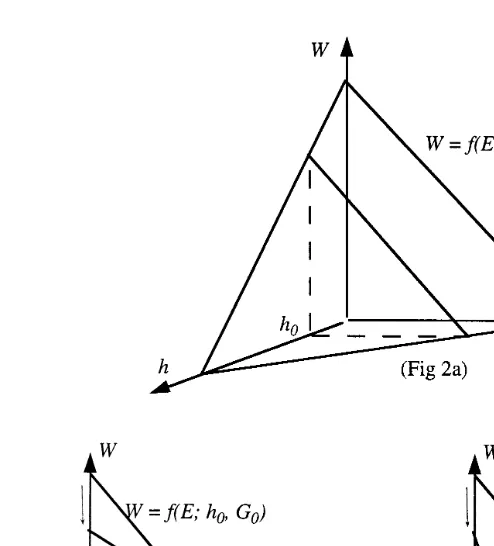
Fig. 2. a Linear labor demand Wsf E; h, G0 for a fixed G ; b If h is also fixed at h , the labor0 0
Ž .
demand curve Wsf E; h , G0 0 obtains. As G increases from G to G , the intercept drops. When0 1
Ž .
dbrdG)0, the curve becomes flatter. c When dbrdG-0, the curve becomes steeper.
Ž ..
and A5 . As noted earlier, these approximations yield the simplest social welfare function needed for comparative statics.12
Ž .
Fig. 2a portrays the labor demand Wsf E; h, G0 with the value of G fixed at G , and Fig. 2b portrays a special case of a two-dimensional demand curve0
Ž .
Wsf E obtained by fixing h at h as well. Note that an increase in G always0
13 Ž
reduces the intercept, because EtrEG-0. With cross-economies of scale i.e.,
. Ž .
EbrEG)0 , an increase in G makes the demand curve flatter Fig. 2b and with
Ž .
cross-diseconomies, steeper Fig. 2c .
12
The negative definiteness of the welfare function is usually assumed. In our model, this condition almost follows from the standard conditions on the cost and production functions. Since our derivation shows that a0)0, b-0, and a4-0, we only need to assume that a2-0. See Footnote 16 for a related discussion.
13
Ž .
Ž . Ž .
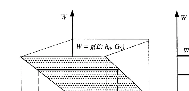
Fig. 3. a Linear labor supply Wsg E; h, G0 for a fixed G . The surface shifts down when G0
Ž . Ž .
increases. b If h is also fixed h , the horizontal supply curve W0 sg E; h , G0 0 obtains. When G increases from G to G , the curve shifts downward.0 1
2.3. Market supply of labor
We abstract from the complexities of the worker’s labor participation decision by specifying the inverse market labor supply function to be of the following form,
Ž .
which is constant with respect to E and parameterized by h, G :
U s
w sg E;h,G
Ž
.
sa0qa1hya2G,Ž .
2where ws is the workers’ asking wage and a0, a1, a2)0 are constants. The simplifying assumption that the supply curve is horizontal,14 shifting downward as either G increases or h decreases, is consistent with the worker’s utility function given earlier in the context of the firm’s problem. For example, when
Ž .
U Y, X, G is linear and a worker takes w, h, and G as fixed, Umax leads to the
Ž .U
same relationship among w, h, and G as in Eq. 2 .
Ž .
Fig. 3a shows the linear labor supply function Wsg E; h, G0 with G fixed at G . If one also fixes h at h , one obtains a horizontal supply curve. This supply0 0
Ž .
curve shifts down when G increases from G to G0 1 Fig. 3b .
14
Ž .
Ž .
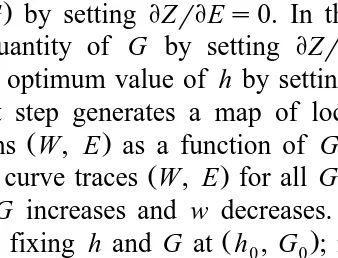
Fig. 4. The equilibrium locus map, where each locus L records the equilibria W, E for a fixed h and all G, h and h are the upper and lower bounds for hour, and hU is the equilibrium hour.
1 3
2.4. Market equilibrium
The competitive market equilibrium is the solution that maximizes the sum total of the surpluses of employers and employees. The process of reaching this equilibrium is illustrated in three steps. First, the market optimizes on E for each
Ž .
fixed h, G by setting EZrEEs0. In the second step, the market chooses the optimum quantity of G by setting EZrEGs0. In the third step, the market chooses the optimum value of h by settingEZrEhs0.
The first step generates a map of locus points for all potential equilibrium
Ž .
combinations W, E as a function of G and h. The result is shown in Fig. 4,
Ž .
where each curve traces W, E for all G and a fixed h. As one moves down on the curve, G increases and w decreases. Fig. 5 depicts a special case of Fig. 4
Ž . Ž .
obtained by fixing h and G at h , G ; it shows the equilibrium point w , E0 0 0 0
Ž . Ž .
[image:10.595.131.300.415.544.2]where the demand and supply curves intersect each other. The second step chooses the optimal point on each curve by equating the marginal social cost of G with its marginal social value.15 The third step selects the optimum hours hU, or the optimum curve L in Fig. 4.2
To understand the curvature in Fig. 4, let us start at a very small value of G
Ži.e., at the top end point of L . As G increases, more workers decide to work2.
and they are willing to work at lower wages than before. As a result, the equilibrium employment increases and the wage decreases, and the curve moves
Ž .
down and to the right. After a certain level of G is reached i.e., beyond point A , benefits become less attractive than before because of the rising marginal non-wage cost of benefits, so a further increase in benefits reduces both the equilibrium employment and the wage, and the curve moves down and to the left.
The above process is equivalent to solving the social welfare maximization
Ž . Ž .
problem summarized by Eq. 4 , with the welfare function 3 specified as
2 Z E, h,G
Ž
.
sa0ya0qŽ
a1ya1.
hqa h22 2
q
Ž
a3qa2.
Gqa G44
EqbŽ
h,G E.
r2qconstant.U
3
Ž .
Ž . Ž . Ž . Ž . Ž .
The optimality conditions appear in Eqs. B1.1 , B1.2 , B1.3 , B2.1 , B2.2 and
ŽB2.3 .. 16
As discussed earlier, the derivative EbrEG represents cross-scale effects. The effect of EbrEG on equilibrium is illustrated in Fig. 4, where h1)h2shU)h3 denote, respectively, the upper bound, the equilibrium level, and the lower bound of hours. The three corresponding L curves are L , L , and L . Moving down the1 2 3 L curve increases G and decreases w. For convenience, Fig. 4 depicts three potential equilibrium points on the curve L . Readers are advised, however, that a2 unique map of locus points is associated with each value of EbrEG, so that only one equilibrium point is relevant on a particular curve. Note also that Fig. 4
Ž .
indicates the maximum employment for each fixed h as being attained at
Ž
equilibrium only whenEbrEGs0 i.e., when the slope of the labor demand curve
.
is constant with respect to G ; otherwise, equilibrium employment is less than the maximum feasible level.
These properties are summarized in the following proposition.
15
Ž . Ž .
By Eqs. B1.2 and B1.3 , the conditions, EZrEhs0 and, EZrEGs0 can be rewritten as
Žaq2 a h E. qŽE2r2.ŽEbrEh.sa E, Ža q2 a G E. qŽE2r2.ŽEbrEG.sya E. The left-hand
1 2 1 3 4 2
Žright-hand sides in both expressions represent the effects of hours and benefits on labor demand. Žsupply . Because the surplus integrates the difference between the demand and supply curves, the.
Ž . Ž .
left-hand right-hand side is interpreted as the marginal social value marginal social cost . 16
The second order condition is consistent with our assumptions on the cost and production functions. When,EbrEhsEbrEGs0, the second order condition is equivalent tob-0, a2-0, and
Ž . Ž .
Proposition 1. a In the absence of cross-scale effects i.e.,EbrEGs0 , competi-tive equilibrium employment is at its maximum feasible level for a given h; however, in the presence of cross-scale effects, equilibrium employment is less
Ž .
than its maximum feasible level; b In the presence of cross-economies of scale
Ži.e., EbrEG)0 , the equilibrium wage lies above that wage associated with.
Ž . Ž .
maximum employment point B in Fig. 4 ; c In the presence of
cross-disecono-Ž .
mies of scale i.e., EbrEG-0 , the equilibrium wage lies below that wage
Ž .
associated with maximum employment point C in Fig. 4 .
Under competition, the market maximizes the sum of the employer and employee
Ž .
surpluses, not employment. In a there are no cross-scale effects and maximizing
Ž . Ž .
surpluses happens to maximize employment. In b and c , however, there are cross-scale effects and maximizing surpluses does not maximize employment.
We proceed to evaluate the effects of an exogenous increase in non-wage benefits on employment, hours, and wages. Increases in G are traced to an
Ž Ž .U.
increase in the demand for G i.e., an increase in a2 in Eq. 2 , to a decrease in
Ž Ž .U. 17
the cost of providing G i.e., an increase in a in Eq. 13 , and an increase in the mandated benefits.
3. Effects of increased demand for G
The demand for benefits may increase if, for example, a new law is introduced that taxes fringe benefits less heavily than wage earnings, or real income grows and fringe benefits are income elastic. An increase in the demand for G is represented by a worker’s willingness to reduce his asking wage, i.e., by an
Ž .U 18
increase in a2 in Eq. 2 . Proposition 2 summarizes our predictions.
Ž .
Proposition 2. Consider the effects on E,G, h of an increase in the demand for G
Ži.e., an increase in a2..
Ž .a IfEbrEGG0, then d Erda2)0, dGrda2)0, and d hŽ rda2.ŽEbrEh.)0;
Ž .b if EbrEG is close toq`, then d Erda2)0, dGrda2)0, and d hrda2 -0;19
17
Note thatya2sdwrdG is the marginal value of G. If G is increased by one unit, a worker is willing to reduce his asking wage bya2 dollars. Thus, an increase in the demand for G results in a
Ž .
downward shift of the horizontal supply curve see Fig. 6 . Similarly, a decrease in the cost of providing G increases the employer’s willingness to pay a higher wage resulting in an upward shift of
Ž .
the negatively sloped demand curve. This change is represented by the dominant factor i.e., a3
ŽU
.
through which affects the demand function 1 . 18
Ž . Ž .
The precise expressions for d Erda2, dGrda2 and d hrda2 appear in Eqs. B6.1 , B6.2 and
ŽB6.3 ..
19
Ž
The expression ‘‘close to q` or y`’’ means that the variable is such a large positive or
.
negative finite number that it outweighs all other constants in the corresponding expressions. For
Ž .
example, the sign ofEbrEh in Eq. A7 is solely determined by C ; however C , cannot be equal to12 12
Ž .c if EbrEG is close toy`, then d Erda2-0, d hrda2-0, and the sign of dGrda2 is ambiguous;
Ž .d ifEbrEG-0 is not very large, then the effects are ambiguous.
Ž .
In a , there may be zero or positive cross-scale effects. In either case, both employment and benefits increase. The intuition behind this result is straightfor-ward. An increase in the demand for benefits is an increase in the marginal value of benefits. An increased demand for benefits makes it welfare enhancing to increase benefits and to decrease the wage in the compensation package. As a result, the equilibrium benefit level rises. This change in the compensation package in turn raises the value of employment to both employers and employees, resulting in an increased employment.
Ž . Ž . Ž .
We illustrate employment effects in b and c using Figs. 2–6. In b , there exist strong cross-economies of scale and employers now prefer giving employees more benefits and lower wages, so an increase in G lowers the intercept and
Ž .
flattens the demand curve Fig. 2b . At the same time, an increase in G shifts
Ž .
down the supply curve, as workers trade off wages for benefits Fig. 3b . As a
Ž .
result, the equilibrium employment increases Fig. 6a . Hours of work decrease, however.
The intuition behind the above result is that increases in benefits and employ-ment reinforce each other because of strong cross-economies of scale, causing
Ž .
benefits and employment to increase more than they do in a . Hours decrease because employers substitute employment for hours and workers reduce hours of
Ž .
work in response to a decline in the wage cf. Proposition 3 .
Ž .
In case c , there exist strong cross-diseconomies of scale, so the increase in G
Ž .
steepens the demand curve and lowers the intercept Fig. 2c , resulting in a
Ž .
decrease in equilibrium employment Fig. 6b . Here, cross-diseconomies of scale
[image:13.595.60.372.391.536.2]Ž . Ž . Ž .
Fig. 6. Effects on W, E of an increase in benefits G1)G . a Employment increases when0
Ž .
generate forces that are opposite to the positive influence on employment
associ-Ž .
ated with case a , and employment ends up falling.
Ž . Ž .
For two reasons, we believe that a and b may be the most relevant cases in understanding the U.S. experience. First, insurance has been the fastest growing component of fringe benefits in recent years with the result that by 1994 it has
Ž .
become the largest benefit component see Table 1 . Second, since large firms enjoy cost advantages in providing insurance, an additional employee reduces the
Ž .
marginal cost of benefits i.e., C12 is negative . These considerations suggest that the secular increase in fringe benefits, to the extent that it is attributable to an increase in the demand for benefits, may have contributed to employment growth. Because wdswssw in equilibrium, the effect of a demand driven change in G on the wage rate w is ascertained from the following equation:
dwrda2sa1
Ž
d hrda2.
y a2Ž
dGrda2.
qG .Ž
11.
Thus, the effect on the wage consists of two components — the term a1 Žd hrda2., which represents the effect operating through work hours, and the term
wa2ŽdGrda2.qG , which represents the effect working through benefits. Thex wage could increase or decrease, depending on cross-scale effects. Predictions about the wage effect are as follows:
Ž
Proposition 3. Consider the wage effect of an increase in the demand for G i.e.,
.
an increase in a2 .
Ž .a IfEbrEGsEbrEhs0, then dwrda2-0;
Ž .b ifEbrEG is close to q`, then dwrda2-0;
Ž .c the wage effect is ambiguous in all other cases.
Ž .
In a , the wage falls because substituting benefits for the wage is mutually
Ž .
beneficial to employers and employees. The wage falls even more in b because strong cross-economies of scale make it attractive to substitute benefits for wages
Ž .
more than in a . Our model does not predict the wage effects in other situations.
4. Effects of decreased cost of G
Non-wage benefits may increase if the cost of providing fringe benefits decreases. A decrease in the cost of G is represented by the employer’s
Ž .U
willingness to increase the wage rate, i.e., by an increase in a3 in Eq. 1 . Intuitively, a decrease in the cost of G should have the same effect as an increase in its demand. Our analysis shows that our intuition is indeed correct. By totally differentiating the first order condition, we obtain the following results:
d Erd a3sd Erda2, d hrd a3sd hrda2, and dGrd a3sdGrda2. 12
In other words, the effect of a decrease in the cost of G is equivalent to the effect of an increase in the demand for G.
The wage effect is evaluated via the following equation:
dwrd a3sa1d hrd a3ya2dGrd a .3
Ž
13.
We, therefore, have the following proposition:
Ž .
Proposition 4. Consider the effects on E,G, h and on w of a decrease in the cost
Ž .
of providing benefits i.e., an increase in a .3
Ž .a If EbrEGsEbrEhs0, then d Erd a3)0, dGrd a3)0, d hrd a3s0, and dwrd a3-0;
Ž .b if EbrEGG0, then d Erd a3)0, dGrd a3)0, and d hŽ rd a3.ŽEbrEh.)0, the wage effect is ambiguous;
Ž .c ifEbrEG is close toq`, then d Erd a3)0, dGrd a3)0, d hrd a3-0, and dwrd a3-0;
Ž .d ifEbrEG is close toy`, then d Erd a3-0 and d hrd a3-0, the effects on the wage and benefits are ambiguous;
Ž .e if EbrEG-0 is not a large number, all effects are ambiguous.
The interpretations of these predictions are similar to those in Propositions 2
Ž . Ž .
and 3, so we will not repeat them. As previously, we posit that b and c may be the most relevant to understanding the U.S. experience. In particular, the postwar growth in insurance, to the extent it is attributable to a decrease in its cost, may well have contributed to employment growth.
5. Effects of government-mandated increase in G
Government mandated benefits have been one of the major contributors to the
Ž .
growth of non-wage payments cf. Fig. 1 . If the government stipulates the minimum quantity of fringe benefits provided by the employer, then G in the previous model is replaced by the mandated level G. As a result, only two
Ž .
endogenous variables, E and h, remain in the maximization problem 4 . In the revised maximization problem, the first and second order conditions are un-changed except that their dimension is reduced from three to two.20 Totally
20
Ž . wŽ . 2x wŽ
The first order conditions are given as follows: i EZrEEsa0ya0q a1ya1 hqa h2 q a3
2 2
. x4 Ž . Ž . wŽ . x Ž .
qa2Gqa G4 qb h, G Es0, ii EZrEhs a1ya1q2 a h E2 q E r2EbrEhs0. The sec-ond order csec-onditions are equivalent to the negative definiteness of the new Hessian matrix,
2 2 2 b ŽEr2.EbrEh
E ZrEE E ZrŽEEEh.
U
H s 2 2 2 s .
Er2 EbrEh 2a E
Ž .
differentiating the first order conditions with respect to G, we obtain the follow-ing:
U
< <
d ErdGs y
Ž
2 a E2 rH.
a2qŽ
a3q2 a G4.
qEŽ
EbrEG.
,Ž
14a.
U
< <
d hrdGs
Ž
Er2 H.
Ž
EbrEh.
a2qŽ
a3q2 a G4.
qEŽ
EbrEG.
s y
Ž
1r4 a2. Ž
EbrEh.
Ž
d ErdG ,.
Ž
14b.
< U< U Ž 20.
where H is the determinant of the new Hessian matrix H Footnote . Note that the sign of d ErdG is the same as
j
Ž .
G ' a3q2 a G4 qEEbrEG y yŽ
a2.
,Ž
15.
where the term in brackets is the effect of G on labor demand, and the term
Žya2. is the effect on labor supply. When there are strong cross-economies or < <
cross-diseconomies of scale, EbrEG is a very large number so that it dominates in
Ž . Ž .
determining the signs of d ErdG and d hrdG in Eqs. 14a and 14b . Now, define G as the value of G associated with the maximum feasible E. In other0 words, G is defined by
j
Ž .
G0 s0, or a3q2 a G4 qEŽ
EbrEG y yŽ
a2.
s0.Ž
16.
Then, by
X
<
j
Ž .
G0 s2 a4qŽ
d ErdG.
EbrEGGsG0s2 a4-0,Ž . Ž .
we d ErdGsj G -0 if G)G and d E0 rdGsj G )0 if G-G . Finally,0 the following equation evaluates the wage effect of an increase in G:
dwrdGsa1
Ž
d hrdG.
ya2,Ž
17.
which depends critically on the sign of d hrdG. Proposition 5 summarizes the above predictions.
Ž .
Proposition 5. Consider the effects on E, h and w of an increase in the
mandated benefit levels, G.
Ž .a If EbrEG is close toq`, then d ErdG)0, d hrdG-0 and dwrdG-0;
Ž .b if EbrEG is close toy`, then d ErdG-0, d hrdG-0 and dwrdG-0;
Ž .c let G be given by Eq. 16 . Then d E0 Ž . rdG-0
m
G)G ; and the effects0 on hours and the wage are ambiguous.Employment effects of a mandated increase in benefits depend on the initial benefit level as well as the cross-scale effects. If there exist strong
cross-econo-Ž . Ž .
mies diseconomies of scale, a mandated increase in G lowers raises the
Ž . Ž
marginal non-wage cost of employment. This flattens Fig. 2b or steepens Fig.
. Ž . Ž .
Ž .
In a , there exist strong cross-economies of scale, so the mandated increase in benefits reduces the marginal non-wage cost of benefits, causing employment to increase at the expense of hours. This prediction is the opposite of what one might expect using the traditional analysis because the traditional analysis ignores the influence of cross-economies of scale.
Ž .
In b , there exist strong cross-diseconomies of scale, and the mandated increase in benefits causes employment and hours to decrease because of a large increase in the marginal non-wage cost of employment. On the other hand, if the
Ž . Ž .
initial benefit levels are ‘‘high’’ ‘‘low’’ , employment decreases increases regardless of cross-scale effects, but the effect on hours cannot be predicted.
Ž . Ž .
In both a and b , the strong cross-scale effects cause d hrdG to be a large
Ž .
negative number. As a result, Eq. 17 is negative, i.e., the wage falls. This result suggests that the recent decline in work hours and the slow wage growth may reflect the effects of increases in mandated benefits.
Ž .
As for c , consider the special case of EbrEGs0. Then G is the competitive0 equilibrium level of benefits for which E is at its maximum feasible level.21 Therefore, employment decreases regardless of whether the government mandates that G be increased or decreased. There is nothing that the government can do to increase employment by regulating G.22
6. Summary
We have conducted a market level analysis to evaluate the effects of increased benefits on employment, hours of work and the wage rate. Our model facilitates an analysis of how employment, hours of work and the wage change in response to an increase in the demand for benefits, to a decrease in the cost of providing benefits, or to an increase in government-mandated benefit levels.
Our analysis shows that employment may increase, rather than decrease, in response to increased non-wage benefits. Our predictions are found to depend critically on cross-scale effects. When there are strong cross-economies of scale, employment increases in response to an increased demand for benefits, to a decreased cost of providing benefits, or to increased government-mandated benefit levels. Furthermore, hours of work and the wage both decrease. If there are zero or small cross-economies of scale, employment and benefits increase, but no clear predictions emerge either for hours or for the wage. When there are strong
21
Ž . Ž .
If EbrEGs0, the first order conditions B1.1 – B1.3 describe a competitive equilibrium in
Ž . w
which employment reaches its maximum level Proposition 1 . In this case, the expression a3q2 a G4 0
x Ž . Ž . Ž .
qE EbrEGy ya2 s0 is equivalent to Eq. B1.3 . The remaining two conditions B1.1 and
ŽB1.2 are satisfied by i and ii in Footnote 20.. Ž . Ž .
22
It should be remembered that government intervention in a competitive labor market reduces
Ž .
cross-diseconomies of scale, employment and hours both decrease, but the effects on benefits and the wage are ambiguous. If there are weak cross-diseconomies, the model generates ambiguous predictions.
Cross-economies of scale seems to be a reasonable assumption, at least for some sectors in the U.S. labor market, where employer-provided insurance cover-age has emerged as not only the fastest growing fringe benefit but also the largest. Cross-economies in insurance are empirically plausible, because larger firms are likely to have lower marginal non-wage costs of benefits. If so, increased fringe benefits due to a number of different shocks might have contributed to, rather than hindered, employment growth during the past several decades in the US and elsewhere.
Several simplifying assumptions have helped make the analysis manageable. Further refinement of the model would enrich the analysis. First, one might model the worker’s decision on how many hours to work. Second, one might generalize the model by specifying the cost of providing benefits to depend on hours of work. Third, one might model workers as heterogeneous with respect to their tastes for fringe benefits and hours in order to generate an upward sloped supply curve.
Many of our predictions are testable in principle. To test them, one would begin
Ž .
by classifying observations i.e., firms, industry sectors, or countries according to cross-scale effects. Then, one would estimate the relationship between the changes
Ž
in the dependent variables i.e., employment, non-wage benefits, hours of work
. Ž
and wages and the changes in the exogenous variables i.e., the demand for
.
benefits, the costs of providing benefits, and government mandates . Such esti-mated relationship would enable one to accept or reject our predictions.
Testing our theory by inter-country comparisons would be useful as well. Different countries have experienced different rates of rising non-wage labor costs. Among some of the OECD countries, for example, between the mid-1960s and the early 1990s the proportion of non-wage labor cost grew by 101% in the UK, 70% in the US, 26% in Japan, 18% in Germany, and 4% in France. A careful examination of the sources of these differences and differences in employment growths would be useful for testing our theory.
Acknowledgements
gratefully acknowledges the 1996 summer support provided by ISER of Osaka University through its Visiting Foreign Scholarship program.
Appendix A. Derivation of market labor demand functions
I. Consider the second order Taylor approximations of F and C, or assume that F and C are both quadratic as follows:
F n, h
Ž
.
sF n2r2q0.5F h2qF nhqu nqu hqu ,11 22 12 1 2 0
C G, n
Ž
.
sC G2r2qC Gnqf Gqf nqf .11 12 1 2 0
ŽNote that C is assumed to be linear in n, or that C22s0. The individual labor.
demand functions then have the following form:
ns
Ž
hwyV.
rD,Ž
A1.
where
DspF11y2 C G
Ž
12 qf2.
,Vsp F
Ž
yF n.
yŽ
C G2r2qf Gqf.
.n 11 11 1 0
Proof: We begin with the following expressions: FnsEFrEFsF n11 qF h12 qu1)0, FhsEFrEhsF h22 qF n12 qu2)0,
and
C1sECrEGsC G11 qC n12 qf1)0, C2sECrEnsC G12 qf240.
Ž .
The inverse demand for employment 10 is now given by ws pFny
Ž
CqnC2.
rh2
s
Ž
1rh.
pFny C G11 r2qC Gn12 qf1Gqf2nqf0 qn C GŽ
12 qf2.
4
s
Ž
1rh.
pFy
Ž
C G2r2qf Gqf.
y2 C GŽ
qf.
n4
n 11 1 0 12 2
s
Ž
1rh.
p FŽ
nyF n11.
yŽ
C G11 2r2qf1Gqf0.
q pF11y2 C G
Ž
12 qf2.
n4
s
Ž
VqDn.
rh so thatns
Ž
1rD. Ž
hwyV.
2
s hwyp F
Ž
nyF n11.
qŽ
C G11 r2qf1Gqf0.
is the individual labor demand function. Note that FnyF n11 sF h12 qu1,
Ž .
so that the right hand side of Eq. A2 is a function of W, parameterized by h, G, and p.
Ž . Ž . Ž . X
II. If i all firms are identical and if ii psp E , p-0, then the inverse market labor demand function has the form
wst
Ž
h,G.
qbŽ
h,G E.
q´Ž
h,G, E ,.
Ž
A3.
where
2
t
Ž
h,G.
s const.yC G11 r2yf1Gqp F h0 12 rh,Ž
A4.
X
b
Ž
h,G.
s const.y2C G12 qKp F hŽ
12 qu1.
rŽ
Kh ,.
Ž
A5.
Ž . w Ž . x
and ´ h, G, E is a residual term. In Eq. A4 , p0)0 is some constant.
Ž . Ž .
Proof: Since psp E is a function of E, the right-hand side of Eq. A2 contains the term E. Thus, the market labor demand function cannot be derived by
Ž .
multiplying Eq. A2 by K ; it is instead derived by rearranging the expression after moving all E the terms to the left-hand side. This is done as follows.
Ž .
Multiplying Eq. A2 by K, we have
EsnKsK hw
Ž
yV.
rDfrom which we derive KhwsDEqKV
sE pF11y2 C G
Ž
12 qf2.
2
qK p F
Ž
nyF n11.
yŽ
C G11 r2qf1Gqf0.
sy
Ž
C G2r2qf Gqf.
Ky2 C GŽ
qf.
EqKF p E .Ž .
11 1 0 12 2 n
Ž . X
Substituting FnsF n11 qF h12 qu1 and p E sp0qp EqPPP into the above expression, we arrive at
2
ws const.yC G11 r2yf1Gqp F h0 12 rh
X
q const.y2C G12 qKp F h
Ž
12 qu1.
ErŽ
Kh.
q´Ž
h,G, E.
st
Ž
h,G.
qbŽ
h,G E.
q´Ž
h,G, E ,.
Ž .
where´ h, G, E is a residual term containing all other higher order terms of E.
Ž . Ž . Ž . Ž
Settingt h, G sa0qa h, G , we have a0sp F0 12)0 and a h, G s const.y
2 . .
C G11 r2yf1Grh . Thus,
EtrEGsy
Ž
C Gqf.
rh, Et2rEG2syC rh-0,Ž
A6.
11 1 11
EtrEhsya h,G rh, Et2r
Eh2s2 a h,G rh2,
Ž
.
Ž
.
w
Xx
2EbrEGsy2C12r
Ž
Kh ,.
EbrEhsy const.y2C G12 qKpu1 rŽ
Kh.
. A7Ž . Ž .U
Note that when Eq. A3 is approximated by Eq. 1
wdsf E;h,G
Ž
.
sa0q
Ž
a h1 qa h2 2.
qŽ
a G3 qa G4 2.
qŽ
b0qb h1 qb G E,2.
where
t
Ž
h,G.
sa qŽ
a hqa h2.
qŽ
a Gqa G2.
,0 1 2 3 4
b
Ž
h,G.
sb0qb h1 qb G,2we have
a0sp F0 12)0, a4syC11rh-0, b0spXF12-0,
a1q2 a h2 fEtrEh, a3q2 a G4 fEtrEG,
and
b1fEbrEh, b2fEbrEGsy2C12r
Ž
Kh ..
The above expressions show that the signs of EbrEh andEbrEG are ambiguous.
Ž .
The assumption that a2-0 is equivalent to the assumption that a h, G -0.
Appendix B. Derivation of the Hessian matrix
Ž .
The first order condition 5 becomes
2 2
EZrEEs
a0ya0qŽ
a1ya1.
hqa h2 qŽ
a3qa2.
Gqa G44
qb
Ž
h,G E.
s0,Ž
B1.1.
2
EZrEhs
Ž
a1ya1.
q2 a h E2 qŽ
E r2.
EbrEhs0,Ž
B1.2.
2
EZrEGs
Ž
a3qa2.
q2 a G E4 qŽ
E r2.
EbrEGs0.Ž
B1.3.
w Ž .
It follows from the above equations and the linear assumption b h, G sb0q
x
b h1 qb G that2
2 2 2 2
E ZrEE E ZrEEEh E ZrEEEG
2 2 2 2
E ZrEhEE E ZrEh E ZrEhEG Hs
2 2 2 2
E ZrEGEE EZrEGEh E ZrEG
b a1ya1q2 a h2 qEEbrEh a3qa2q2 a G4 qEEbrEG
2 2 2 2 2
aya q2 a hqEEbrEh 2 a EqŽE r2.EbrEh ŽE r2.EbrEhEG
s 1 1 2 2
2 2 2 2 2
a3qa2q2 a G4 qEEbrEG ŽE r2.EbrEhEG 2 a E4 qŽE r2.EbrEh
b ŽEr2.EbrEh ŽEr2.EbrEG Er2EbrEh 2 a E 0
Ž .
s 2 .
Er2EbrEG 0 2 a E
The negative definiteness of H is then equivalent to the following:
E2ZrEE2sb-0, E2ZrEh2s2 a E-0, E2ZrEG2s2 a E-0;
Ž
B2.1.
2 4
2 2
2 2 2 2 2
E ZrEE E ZrEh y E ZrEEEh s2 a bEy
Ž
Er2EbrEh.
)0,Ž
. Ž
.
Ž
.
2B2.2
Ž
.
2 2
2 2 2 2 2
E ZrEE E ZrEG y E ZrEEEG s2 a bEy
Ž
Er2EbrEG.
)0,Ž
. Ž
.
Ž
.
42
2 2 2 2 2 2
E ZrEh E ZrEG y E ZrEhEG s4 a a E )0;
Ž
. Ž
.
Ž
.
2 42 2
2 3 3
Hs4 a a2 4bE y
Ž
a E4 r2.
Ž
EbrEh.
yŽ
a E2 r2.
Ž
EbrEG.
-0. B2.3Ž
.
Ž .
Proof of Proposition 1: By fixing h, solving Eq. B1.1 for E, and computing d ErdGs0 to select the point of maximum employment, we obtain
a3qa2q2 a G4 qEEbrEGs0.
Ž
B3.
We then obtain the point on the L curve corresponding to a competitive
equilib-Ž . Ž .
rium by combining Eqs. B1.1 and B1.3 to arrive at
a3qa2q2 a G4 q
Ž
Er2.
EbrEGs0.Ž
B4.
Ž . Ž .
Clearly, Eqs. B3 and B4 are equivalent only when EbrEGs0. Therefore, the competitive equilibrium level of employment corresponds to the maximum level of employment only when EbrEGs0.
Ž . Ž .
We now demonstrate parts b and c of this proposition. We first rearrange
Ž .
Eq. B1.3 to obtain
y
Ž
a3qa2q2 a G4.
sŽ
Er2.
EbrEG.Ž
B5.
Given that a4-0, an increase in G increases both the right- and left-hand sides of
Ž .
Eq. B5 . Because we impose a linearity assumption on b,EbrEG is a constant. If EbrEG)0, the right-hand-side increases only when E increases. This result implies that we are at point B in Fig. 4 where the current equilibrium wage wB exceeds wU, the equilibrium wage when employment is at its maximum with respect to hU. Similarly, ifEbrEG-0, E falls when G increases. In this case, we are at point C in Fig. 4. This completes the proof of Proposition 1.
Proof of Proposition 2: By totally differentiating the first order conditions given
Ž . Ž . Ž . Ž .
by Eq. 5 or Eqs. B1.1 , B1.2 and B1.3 , we obtain the following comparative statics:
2
w
x
d Erda2s
Ž
a E2 r H.
y4 a G4 qEEbrEGŽ
B6.1.
2
w
x
d hrda2s y
Ž
E r4 H.
Ž
EbrEh.
y4 a G4 qEEbrEGs y
Ž
1r4 a2. Ž
EbrEh. Ž
d Era2.
,Ž
B6.2.
2 2
dGrda2s y
Ž
E r H.
½
2 a2byŽ
Er4. Ž
EbrEh.
ya G2 EbrEG ,5
B6.3< < < < where H is the determinant of the Hessian matrix, H. Because a and H2 -0, d Erda2 has the same sign as
y4 a G4 qEEbrEG,
Ž
B7.
while dGrda2 has the same sign as
2
2 a2by
Ž
Er4. Ž
EbrEh.
ya G2 EbrEG.Ž
B8.
Ž . Ž .Ž .2
It then follows from Eq. B2.2 that 2 a2by Er4 EbrEh )0. Because a2-0
Ž . Ž .
and a4-0, both Eqs. B7 and B8 are positive when EbrEGG0. The effect on
Ž .
hours follows directly from Eq. B6.2 and from the fact that EbrEhF0 when
Ž
EbrEG is a very large positive number i.e., C12 is a very large negative number,
Ž ..
see Eq. A7 . This proves the first two parts of Proposition 2. IfEbrEG is a very
Ž . Ž .
large negative number i.e., C12 is a very large positive number , Eq. A7 implies
Ž . Ž .
that EbrEh is positive. Thus, by Eqs. B6.1 and B6.2 , d Erda2-0 and d hrda2-0. This completes the proof of Proposition 2.
Ž . Ž .
Proof of Proposition 3: The conclusions follow from Eq. 11 and parts a and
Ž .b of Proposition 2.
Ž . Ž .
Proof of Proposition 4: The conclusions follow from Eqs. 12 and 13 as well as Propositions 2 and 3.
Ž .
Proof of Proposition 5: When EbrEG is close toq` i.e., C12 is close toy`,
Ž . Ž . Ž .
Eqs. A7 , 14a and 14b jointly imply d ErdG)0 and d hrdG because a2-0,
U
<H <)0, and EbrEh-0. Similarly, when EbrEG is close to y`, d ErdG-0
Ž .
and d hrdG-0. Since d hrdG-0 holds in both cases, it follows from Eq. 17
Ž .
that dwrdG is negative. Part c follows from the discussion preceding the proposition. This completes the proof of our last proposition.
References
Brechling, F., 1977. The Incentive Effects of the US Unemployment Insurance Tax. In: Research in Labor Economics, Vol. 1, Jai Press, Greenwich, CT.
Chamber of Commerce of the United States, 1981. Employee Benefits Historical Data, 1951–1979. U.S. Chamber of Commerce, Washington, DC.
Chamber of Commerce of the United States, 1985, 1989, 1993, 1994, 1995. Employee Benefits. U.S. Chamber of Commerce, Washington, DC.
Congress of the United States — Congressional Budget Office, 1992. Economic Implications of Rising Health Care Costs, October.
Ehrenberg, R.G., 1971. Fringe Benefits and Overtime Behavior. Lexington Books, Lexington. Hamermesh, D.S., 1993. Labor Demand. Princeton Univ. Press, Princeton.
Hart, R.A., D. Bell, R. Frees, S. Kawsaki, S.A. Woodbury, 1988. Trends in Non-Wage Labor Costs and Their Effects on Employment, Final Report. Brussels–Luxembourg Commission of the European Communities.
Hashimoto, M., 1994. The Effects of Non-Wage Compensation on Employment and Hours, a paper presented to the Upjohn Institute Conference on Employment Benefits, Labor Costs, and Labor Markets in Canada and the United States, November.
Nadiri, M.I., Rosen, S., 1969. Interrelated factor demand functions. American Economic Review 59, 457–471.
Oi, W., 1962. Labor as a quasi-fixed factor. Journal of Political Economy 70, 538–555.
Rosen, S., 1968. Short-employment variation on Class-I railroads in the US, 1947–1963. Econometrica 36, 511–529.
United States Department of Labor, Bureau of Labor Statistics, 1977. Employee Compensation in the Private Nonfarm Economy, 1974. Bulletin No. 1963, USGPO, Washington, DC.
United States Department of Labor, Bureau of Labor Statistics, 1995. Employer Costs for Employee
Ž
Compensation, March 1995. News Release No. 95-0272 USDL, Bureau of Labor Statistics,
.
Washington, DC; Available at the Web site: http:rrstats.bls.govrnews.releaserecec.toc.htm . Woodbury, S.A., 1983. Substitution between wage and nonwage benefits. American Economic Review