MATLAB, 4th Edition ebook free download

(1)

(2)

(3)

M

ATLAB

®

An Introduction

(4)

(5)

M

ATLAB

®

An Introduction

with Applications

Fourth Edition

Amos Gilat

Department of Mechanical Engineering

The Ohio State University

(6)

MARKETING MANAGER Christopher Ruel EDITORIAL ASSISTANT Katie Singleton

DESIGNER Wendy Lai

MEDIA EDITOR Thomas Kulesa

PRODUCTION MANAGER Micheline Frederick PRODUCTION EDITOR Amy Weintraub Cover images: Amos Gilat

This book was printed and bound by Malloy Lithographers. The cover was printed by Malloy Lithographers.

This book is printed on acid free paper.

Copyright © 2011 John Wiley & Sons, Inc. All rights reserved. No part of this publi-cation may be reproduced, stored in a retrieval system or transmitted in any form or by any means, electronic, mechanical, photocopying, recording, scanning or other-wise, except as permitted under Sections 107 or 108 of the 1976 United States Copy-right Act, without either the prior written permission of the Publisher, or authorization through payment of the appropriate per-copy fee to the Copyright Clearance Center, Inc. 222 Rosewood Drive, Danvers, MA 01923, website www.copyright.com. Requests to the Publisher for permission should be addressed to the Permissions Department, John Wiley & Sons, Inc., 111 River Street, Hoboken, NJ 07030-5774, (201)748-6011, fax (201)748-6008, website http://www.wiley.com/go/permissions. "Evaluation copies are provided to qualified academics and professionals for review purposes only, for use in their courses during the next academic year. These copies are licensed and may not be sold or transferred to a third party. Upon completion of the review period, please return the evaluation copy to Wiley. Return instructions and a free of charge return shipping label are available at www.wiley.com/go/returnlabel. Outside of the United States, please contact your local representative."

Library of Congress Cataloging in Publication Data:

ISBN-13 978-0-470-76785-6

Printed in the United States of America 10 9 8 7 6 5 4 3 2 1

(7)

v

Preface

MATLAB® is a very popular language for technical computing used by stu-dents, engineers, and scientists in universities, research institutes, and industries all over the world. The software is popular because it is powerful and easy to use. For university freshmen in it can be thought of as the next tool to use after the graphic calculator in high school.

This book was written following several years of teaching the software to freshmen in an introductory engineering course. The objective was to write a book that teaches the software in a friendly, non-intimidating fashion. Therefore, the book is written in simple and direct language. In many places bullets, rather than lengthy text, are used to list facts and details that are related to a specific topic. The book includes numerous sample problems in mathematics, science, and engi-neering that are similar to problems encountered by new users of MATLAB.

This fourth edition of the book is updated to MATLAB 7.11 (Release 2010b). Other modifications/changes to this edition are: programming (now Chapter 6) is introduced before user-defined functions (now Chapter 7), applica-tions in numerical analysis (now Chapter 9) follows polynomials, curve fitting and interpolation that is covered in Chapter 8. The last two chapters are 3D plot-ting (now Chapter 10) and symbolic math (Chapter 11). In addition, the end of chapter problems have been revised. There are many more problems in every chapter, and close to 80% are new of different than in previous editions. In addi-tion, the problems cover a wider range of topics.

I would like to thank several of my colleagues at The Ohio State University. Professors Richard Freuler, Mark Walter, and Walter Lampert, and Dr. Mike Parke read sections of the book and suggested modifications. I also appreciate the involvement and support of Professors Robert Gustafson and John Demel and Dr. John Merrill from the First-Year Engineering Program at The Ohio State Univer-sity. Special thanks go to Professor Mike Lichtensteiger (OSU), and my daughter Tal Gilat (Marquette University), who carefully reviewed the first edition of the book and provided valuable comments and criticisms. Professor Brian Harper (OSU) has made a significant contribution to the new end of chapter problems in the present edition.

(8)

of Iowa; Brian Vick, Virginia Polytechnic Institute and State University; Jay Weitzen, University of Massachusetts, Lowell; and Jane Patterson Fife, The Ohio State University. In addition, I would like to acknowledge Daniel Sayre, Ken San-tor, and Katie Singleton, all from John Wiley & Sons, who supported the produc-tion of the Fourth ediproduc-tion.

I hope that the book will be useful and will help the users of MATLAB to enjoy the software.

Amos Gilat Columbus, Ohio November, 2010 gilat.1@osu.edu

(9)

vii

Preface

v

Introduction

1

Chapter 1

Starting with MATLAB

5

1.1 STARTING MATLAB, MATLAB WINDOWS 5

1.2 WORKING IN THE COMMAND WINDOW 9

1.3 ARITHMETIC OPERATIONS WITH SCALARS 10

1.3.1 Order of Precedence 11

1.3.2 Using MATLAB as a Calculator 11

1.4 DISPLAY FORMATS 12

1.5 ELEMENTARY MATH BUILT-IN FUNCTIONS 13

1.6 DEFINING SCALAR VARIABLES 16

1.6.1 The Assignment Operator 16

1.6.2 Rules About Variable Names 18

1.6.3 Predefined Variables and Keywords 18

1.7 USEFUL COMMANDS FOR MANAGING VARIABLES 19

1.8 SCRIPT FILES 20

1.8.1 Notes About Script Files 20

1.8.2 Creating and Saving a Script File 21

1.8.3 Running (Executing) a Script File 22

1.8.4 Current Folder 22

1.9 EXAMPLES OF MATLAB APPLICATIONS 24

1.10 PROBLEMS 27

Chapter 2

Creating Arrays

35

2.1 CREATING A ONE-DIMENSIONAL ARRAY (VECTOR) 35

2.2 CREATING A TWO-DIMENSIONAL ARRAY (MATRIX) 39

2.2.1 The zeros, ones and, eye Commands 40

2.3 NOTES ABOUT VARIABLES IN MATLAB 41

2.4 THE TRANSPOSE OPERATOR 41

2.5 ARRAY ADDRESSING 42

2.5.1 Vector 42

2.5.2 Matrix 43

2.6 USING A COLON : IN ADDRESSING ARRAYS 44

2.7 ADDING ELEMENTS TO EXISTING VARIABLES 46

2.8 DELETING ELEMENTS 48

2.9 BUILT-IN FUNCTIONS FOR HANDLING ARRAYS 49

2.10 STRINGS AND STRINGS AS VARIABLES 53

2.11 PROBLEMS 55

Chapter 3

Mathematical Operations with Arrays

63

3.1 ADDITION AND SUBTRACTION 64

3.2 ARRAY MULTIPLICATION 65

(10)

3.4 ELEMENT-BY-ELEMENT OPERATIONS 72

3.5 USING ARRAYS IN MATLAB BUILT-IN MATH FUNCTIONS 75

3.6 BUILT-IN FUNCTIONS FOR ANALYZING ARRAYS 75

3.7 GENERATION OF RANDOM NUMBERS 77

3.8 EXAMPLES OF MATLAB APPLICATIONS 80

3.9 PROBLEMS 86

Chapter 4

Using Script Files and Managing Data

95

4.1 THE MATLAB WORKSPACE AND THE WORKSPACE WINDOW 96

4.2 INPUT TO A SCRIPT FILE 97

4.3 OUTPUT COMMANDS 100

4.3.1 The disp Command 101

4.3.2 The fprintf Command 103

4.4 THE save AND load COMMANDS 111

4.4.1 The save Command 111

4.4.2 The load Command 112

4.5 IMPORTING AND EXPORTING DATA 114

4.5.1 Commands for Importing and Exporting Data 114

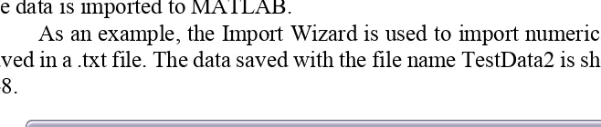
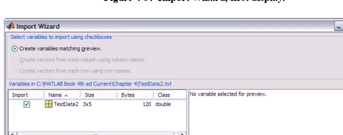
4.5.2 Using the Import Wizard 116

4.6 EXAMPLES OF MATLAB APPLICATIONS 118

4.7 PROBLEMS 123

Chapter 5

Two-Dimensional Plots

133

5.1 THE plot COMMAND 134

5.1.1 Plot of Given Data 138

5.1.2 Plot of a Function 139

5.2 THE fplot COMMAND 140

5.3 PLOTTING MULTIPLE GRAPHS IN THE SAME PLOT 141

5.3.1 Using the plot Command 141

5.3.2 Using the hold on and hold off Commands 142

5.3.3 Using the line Command 143

5.4 FORMATTING A PLOT 144

5.4.1 Formatting a Plot Using Commands 144

5.4.2 Formatting a Plot Using the Plot Editor 148

5.5 PLOTS WITH LOGARITHMIC AXES 149

5.6 PLOTS WITH ERROR BARS 150

5.7 PLOTS WITH SPECIAL GRAPHICS 152

5.8 HISTOGRAMS 153

5.9 POLAR PLOTS 156

5.10 PUTTING MULTIPLE PLOTS ON THE SAME PAGE 157

5.11 MULTIPLE FIGURE WINDOWS 157

(11)

Contents

ix

Chapter 6

Programming in MATLAB

173

6.1 RELATIONAL AND LOGICAL OPERATORS 174

6.2 CONDITIONAL STATEMENTS 182

6.2.1 The if-end Structure 182

6.2.2 The if-else-end Structure 184

6.2.3 The if-elseif-else-end Structure 185

6.3 THE switch-case STATEMENT 187

6.4 LOOPS 190

6.4.1 for-end Loops 190

6.4.2 while-end Loops 195

6.5 NESTED LOOPS AND NESTED CONDITIONAL STATEMENTS 198

6.6 THE break AND continue COMMANDS 200

Chapter 7

User-Defined Functions and Function Files

219

7.1 CREATING A FUNCTION FILE 220

7.2 STRUCTURE OF A FUNCTION FILE 221

7.2.1 Function Definition Line 222

7.2.2 Input and Output Arguments 222

7.2.3 The H1 Line and Help Text Lines 224

7.2.4 Function Body 224

7.3 LOCAL AND GLOBAL VARIABLES 224

7.4 SAVING A FUNCTION FILE 225

7.5 USING A USER-DEFINED FUNCTION 226

7.6 EXAMPLES OF SIMPLE USER-DEFINED FUNCTIONS 227

7.7 COMPARISON BETWEEN SCRIPT FILES AND FUNCTION FILES 229

7.8 ANONYMOUS AND INLINE FUNCTIONS 229

7.8.1 Anonymous Functions 230

7.8.2 Inline Functions 233

7.9 FUNCTION FUNCTIONS 234

7.9.1 Using Function Handles for Passing a Function into a Function

Function 235

7.9.2 Using a Function Name for Passing a Function into a Function

Function 238

7.10 SUBFUNCTIONS 240

7.11 NESTED FUNCTIONS 242

7.13 PROBLEMS 248

Chapter 8

Polynomials, Curve Fitting, and Interpolation

261

8.1 POLYNOMIALS 261

8.1.1 Value of a Polynomial 262

8.1.2 Roots of a Polynomial 263

8.1.3 Addition, Multiplication, and Division of Polynomials 264

8.1.4 Derivatives of Polynomials 266

(12)

8.2.1 Curve Fitting with Polynomials; The polyfit Function 267

8.2.2 Curve Fitting with Functions Other than Polynomials 271

8.3 INTERPOLATION 274

8.4 THE BASIC FITTING INTERFACE 278

Chapter 9

Applications in Numerical Analysis

295

9.1 SOLVING AN EQUATION WITH ONE VARIABLE 295

9.2 FINDING A MINIMUM OR A MAXIMUM OF A FUNCTION 298

9.3 NUMERICAL INTEGRATION 300

9.4 ORDINARY DIFFERENTIAL EQUATIONS 303

Chapter 10

Three-Dimensional Plots

323

10.1 LINE PLOTS 323

10.2 MESH AND SURFACE PLOTS 324

10.3 PLOTS WITH SPECIAL GRAPHICS 331

10.4 THE view COMMAND 333

10.6 PROBLEMS 341

Chapter 11

Symbolic Math

347

11.1 SYMBOLIC OBJECTS AND SYMBOLIC EXPRESSIONS 348

11.1.1 Creating Symbolic Objects 348

11.1.2 Creating Symbolic Expressions 350

11.1.3 The findsym Command and the Default Symbolic

Variable 353

11.2 CHANGING THE FORM OF AN EXISTING SYMBOLIC EXPRESSION 354

11.2.1 The collect, expand, and factor Commands 354

11.2.2 The simplify and simple Commands 356

11.2.3 The pretty Command 357

11.3 SOLVING ALGEBRAIC EQUATIONS 358

11.4 DIFFERENTIATION 363

11.5 INTEGRATION 365

11.6 SOLVING AN ORDINARY DIFFERENTIAL EQUATION 366

11.7 PLOTTING SYMBOLIC EXPRESSIONS 369

11.8 NUMERICAL CALCULATIONS WITH SYMBOLIC EXPRESSIONS 372

11.10 PROBLEMS 384

Appendix:

Summary of Characters, Commands, and

Functions

393 Answers to Selected Problems

401

(13)

1 Introduction

MATLAB is a powerful language for technical computing. The name MATLAB stands for MATrix LABoratory, because its basic data element is a matrix (array). MATLAB can be used for math computations, modeling and simulations, data analysis and processing, visualization and graphics, and algorithm development.

MATLAB is widely used in universities and colleges in introductory and advanced courses in mathematics, science, and especially engineering. In industry the software is used in research, development, and design. The standard MATLAB program has tools (functions) that can be used to solve common problems. In addition, MATLAB has optional toolboxes that are collections of specialized programs designed to solve specific types of problems. Examples include toolboxes for signal processing, symbolic calculations, and control systems.

Until recently, most of the users of MATLAB have been people with previous knowledge of programming languages such as FORTRAN and C who switched to MATLAB as the software became popular. Consequently, the majority of the literature that has been written about MATLAB assumes that the reader has knowledge of computer programming. Books about MATLAB often address advanced topics or applications that are specialized to a particular field. Today, however, MATLAB is being introduced to college students as the first (and often the only) computer program they will learn. For these students there is a need for a book that teaches MATLAB assuming no prior experience in computer programming.

The Purpose of This Book

MATLAB: An Introduction with Applications is intended for students who are using MATLAB for the first time and have little or no experience in computer programming. It can be used as a textbook in freshmen engineering courses or in workshops where MATLAB is being taught. The book can also serve as a reference in more advanced science and engineering courses where MATLAB is used as a tool for solving problems. It also can be used for self-study of MATLAB by students and practicing engineers. In addition, the book can be a supplement or a secondary book in courses where MATLAB is used but the instructor does not have the time to cover it extensively.

Topics Covered

(14)

assumption is that once these foundations are well understood, the student will be able to learn advanced topics easily by using the information in the Help menu.

The order in which the topics are presented in this book was chosen carefully, based on several years of experience in teaching MATLAB in an introductory engineering course. The topics are presented in an order that allows the student to follow the book chapter after chapter. Every topic is presented completely in one place and then used in the following chapters.

The first chapter describes the basic structure and features of MATLAB and how to use the program for simple arithmetic operations with scalars as with a calculator. Script files are introduced at the end of the chapter. They allow the student to write, save, and execute simple MATLAB programs. The next two chapters are devoted to the topic of arrays. MATLAB’s basic data element is an array that does not require dimensioning. This concept, which makes MATLAB a very powerful program, can be a little difficult to grasp for students who have only limited knowledge of and experience with linear algebra and vector analysis. The concept of arrays is introduced gradually and then explained in extensive detail. Chapter 2 describes how to create arrays, and Chapter 3 covers mathematical operations with arrays.

Following the basics, more advanced topics that are related to script files and input and output of data are presented in Chapter 4. This is followed by coverage of two-dimensional plotting in Chapter 5. Programming with MATLAB is introduced in Chapter 6. This includes flow control with conditional statements and loops. User-defined functions, anonymous functions, and function functions are covered next in Chapter 7. The coverage of function files (user-defined functions) is intentionally separated from the subject of script files. This has proven to be easier to understand by students who are not familiar with similar concepts from other computer programs.

The next three chapters cover more advanced topics. Chapter 8 describes how MATLAB can be used for carrying out calculations with polynomials, and how to use MATLAB for curve fitting and interpolation. Chapter 9 covers applications of MATLAB in numerical analysis. It includes solving nonlinear equations, finding minimum or a maximum of a function, numerical integration, and solution of first-order ordinary differential equations. Chapter 10 describes how to produce three-dimensional plots, an extension of the chapter on two-dimensional plots. Chapter 11 covers in great detail how to use MATLAB in symbolic operations.

The Framework of a Typical Chapter

(15)

Introduction

3

tutorials in order to gain experience in using MATLAB. In addition, every chapter includes formal sample problems that are examples of applications of MATLAB for solving problems in math, science, and engineering. Each example includes a problem statement and a detailed solution. Some sample problems are presented in the middle of the chapter. All of the chapters (except Chapter 2) have a section at the end with several sample problems of applications. It should be pointed out that problems with MATLAB can be solved in many different ways. The solutions of the sample problems are written such that they are easy to follow. This means that in many cases the problem can be solved by writing a shorter, or sometimes “trickier,” program. The students are encouraged to try to write their own solu-tions and compare the end results. At the end of each chapter there is a set of homework problems. They include general problems from math and science and problems from different disciplines of engineering.

Symbolic Calculations

MATLAB is essentially a software for numerical calculations. Symbolic math operations, however, can be executed if the Symbolic Math toolbox is installed. The Symbolic Math toolbox is included in the student version of the software and can be added to the standard program.

Software and Hardware

The MATLAB program, like most other software, is continually being developed and new versions are released frequently. This book covers MATLAB Version 7.11, Release 2010b. It should be emphasized, however, that the book covers the basics of MATLAB, which do not change much from version to version. The book covers the use of MATLAB on computers that use the Windows operating system. Everything is essentially the same when MATLAB is used on other machines. The user is referred to the documentation of MATLAB for details on using MATLAB on other operating systems. It is assumed that the software is installed on the computer, and the user has basic knowledge of operating the computer.

The Order of Topics in the Book

(16)

(17)

5

Chapter 1 Starting with

MATLAB

This chapter begins by describing the characteristics and purposes of the different windows in MATLAB. Next, the Command Window is introduced in detail. This chapter shows how to use MATLAB for arithmetic operations with scalars in a fashion similar to the way that a calculator is used. This includes the use of ele-mentary math functions with scalars. The chapter then shows how to define scalar variables (the assignment operator) and how to use these variables in arithmetic calculations. The last section in the chapter introduces script files. It shows how to write, save, and execute simple MATLAB programs.

1.1 S

TARTING

MATLAB, MATLAB W

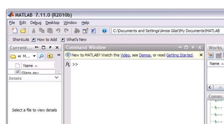
INDOWS

It is assumed that the software is installed on the computer, and that the user can start the program. Once the program starts, the MATLAB desktop window opens (Figure 1-1). The window contains four smaller windows: the Command Window, the Current Folder Window, the Workspace Window, and the Command History Window. This is the default view that shows four of the various windows of MAT-LAB. A list of several windows and their purpose is given in Table 1-1. The Start

button on the lower left side can be used to access MATLAB tools and features. Four of the windows—the Command Window, the Figure Window, the Editor Window, and the Help Window—are used extensively throughout the book and are briefly described on the following pages. More detailed descriptions are included in the chapters where they are used. The Command History Window, Current Folder Window, and the Workspace Window are described in Sections 1.2, 1.8.4, and 4.1, respectively.

Command Window: The Command Window is MATLAB’s main window and

(18)

selecting Command Window Only from the submenu that opens. Working in the Command Window is described in detail in Section 1.2.

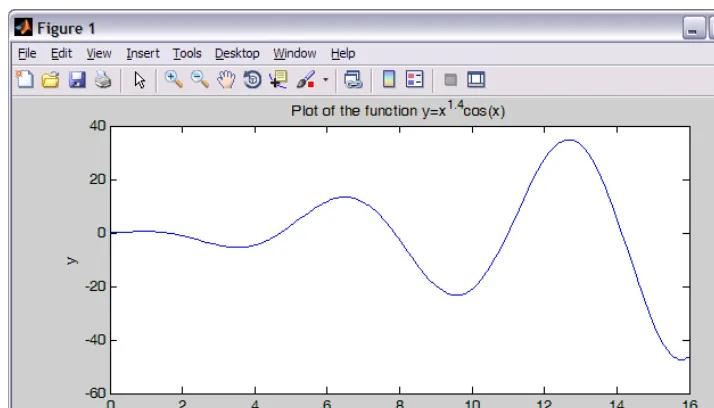
Figure Window: The Figure Window opens automatically when graphics

com-mands are executed, and contains graphs created by these comcom-mands. An example of a Figure Window is shown in Figure 1-2. A more detailed description of this window is given in Chapter 5.

Figure 1-1: The default view of MATLAB desktop. Table 1-1: MATLAB windows

Window Purpose

Command Window Main window, enters variables, runs

programs.

Figure Window Contains output from graphic

commands.

Editor Window Creates and debugs script and

function files.

Help Window Provides help information.

Command History Window Logs commands entered in the

Command Window.

Workspace Window Provides information about the

variables that are used.

(19)

1.1 Starting MATLAB, MATLAB Windows

7

Editor Window: The Editor Window is used for writing and editing programs.

This window is opened from the File menu. An example of an Editor Window is shown in Figure 1-3. More details on the Editor Window are given in Section 1.8.2, where it is used for writing script files, and in Chapter 7, where it is used to write function files.

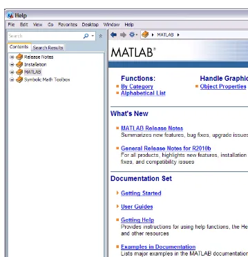
Help Window: The Help Window contains help information. This window can

be opened from the Help menu in the toolbar of any MATLAB window. The Help Window is interactive and can be used to obtain information on any feature of MATLAB. Figure 1-4 shows an open Help Window.

Figure 1-2: Example of a Figure Window.

(20)

When MATLAB is started for the first time the screen looks like that shown in Figure 1-1. For most beginners it is probably more convenient to close all the win-dows except the Command Window. (Each of the winwin-dows can be closed by clicking on the button.) The closed windows can be reopened by selecting them from the Desktop menu. The windows shown in Figure 1-1 can be displayed by selecting first Desktop Layout in the Desktop menu and then Default from the submenu. The various windows in Figure 1-1 are docked to the desktop. A window can be undocked (become a separate, independent window) by clicking

on the button on the upper right-hand corner. An independent window can be redocked by clicking on the button.

(21)

1.2 Working in the Command Window

9 1.2 W

ORKINGINTHE

C

OMMAND

W

INDOW

The Command Window is MATLAB’s main window and can be used for execut-ing commands, openexecut-ing other windows, runnexecut-ing programs written by the user, and managing the software. An example of the Command Window, with several sim-ple commands that will be explained later in this chapter, is shown in Figure 1-5.

Notes for working in the Command Window:

• To type a command the cursor must be placed next to the command prompt ( >> ).

• Once a command is typed and the Enter key is pressed, the command is executed. However, only the last command is executed. Everything executed previously (that might be still displayed) is unchanged.

• Several commands can be typed in the same line. This is done by typing a comma between the commands. When the Enter key is pressed the commands are exe-cuted in order from left to right.

• It is not possible to go back to a previous line that is displayed in the Command Window, make a correction, and then re-execute the command.

• A previously typed command can be recalled to the command prompt with the up-arrow key ( ). When the command is displayed at the command prompt, it can be modified if needed and then executed. The down-arrow key ( ) can be used to move down the list of previously typed commands.

• If a command is too long to fit in one line, it can be continued to the next line by typing three periods … (called an ellipsis) and pressing the Enter key. The tinuation of the command is then typed in the new line. The command can con-tinue line after line up to a total of 4,096 characters.

Figure 1-5: The Command Window.

(22)

The semicolon ( ; ):

When a command is typed in the Command Window and the Enter key is

pressed, the command is executed. Any output that the command generates is dis-played in the Command Window. If a semicolon ( ; ) is typed at the end of a com-mand the output of the comcom-mand is not displayed. Typing a semicolon is useful when the result is obvious or known, or when the output is very large.

If several commands are typed in the same line, the output from any of the commands will not be displayed if a semicolon is typed between the commands instead of a comma.

Typing %:

When the symbol % (percent) is typed at the beginning of a line, the line is desig-nated as a comment. This means that when the Enter key is pressed the line is not executed. The % character followed by text (comment) can also be typed after a command (in the same line). This has no effect on the execution of the command. Usually there is no need for comments in the Command Window. Comments, however, are frequently used in a program to add descriptions or to explain the program (see Chapters 4 and 6).

Theclccommand:

The clc command (type clc and press Enter) clears the Command Window. After working in the Command Window for a while, the display may become very long. Once the clc command is executed a clear window is displayed. The com-mand does not change anything that was done before. For example, if some vari-ables were defined previously (see Section 1.6), they still exist and can be used. The up-arrow key can also be used to recall commands that were typed before.

The Command History Window:

The Command History Window lists the commands that have been entered in the Command Window. This includes commands from previous sessions. A com-mand in the Comcom-mand History Window can be used again in the Comcom-mand Win-dow. By double-clicking on the command, the command is reentered in the Command Window and executed. It is also possible to drag the command to the Command Window, make changes if needed, and then execute it. The list in the Command History Window can be cleared by selecting the lines to be deleted and then selecting Delete Selection from the Edit menu (or right-click the mouse when the lines are selected and then choose Delete Selection in the menu that opens).

1.3 A

RITHMETIC

O

PERATIONSWITH

S

CALARS

(23)

opera-1.3 Arithmetic Operations with Scalars

11

tions are:

It should be pointed out here that all the symbols except the left division are the same as in most calculators. For scalars, the left division is the inverse of the right division. The left division, however, is mostly used for operations with arrays, which are discussed in Chapter 3.

1.3.1 Order of Precedence

MATLAB executes the calculations according to the order of precedence dis-played below. This order is the same as used in most calculators.

In an expression that has several operations, higher-precedence operations are executed before lower-precedence operations. If two or more operations have the same precedence, the expression is executed from left to right. As illustrated in the next section, parentheses can be used to change the order of calculations.

1.3.2 Using MATLAB as a Calculator

The simplest way to use MATLAB is as a calculator. This is done in the Com-mand Window by typing a mathematical expression and pressing the Enter key. MATLAB calculates the expression and responds by displaying ans= and the numerical result of the expression in the next line. This is demonstrated in Tutorial 1-1.

Operation Symbol Example

Addition + 5 + 3

Subtraction – 5 – 3

Multiplication * 5 * 3

Right division / 5 / 3

Left division \ 5 \ 3 = 3 / 5

Exponentiation ^ 5 ^ 3 (means 53

= 125)

Precedence Mathematical Operation

First Parentheses. For nested parentheses, the innermost

are executed first.

Second Exponentiation.

Third Multiplication, division (equal precedence).

(24)

1.4 D

ISPLAY

F

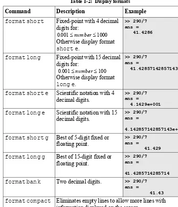
ORMATS

The user can control the format in which MATLAB displays output on the screen. In Tutorial 1-1, the output format is fixed-point with four decimal digits (called short), which is the default format for numerical values. The format can be changed with the format command. Once the format command is entered, all the output that follows is displayed in the specified format. Several of the avail-able formats are listed and described in Tavail-able 1-2.

MATLAB has several other formats for displaying numbers. Details of these formats can be obtained by typing helpformat in the Command Window. The format in which numbers are displayed does not affect how MATLAB computes and saves numbers.

Tutorial 1-1: Using MATLAB as a calculator.

>> 7+8/2 ans = 11 >> (7+8)/2 ans = 7.5000 >> 4+5/3+2 ans = 7.6667 >> 5^3/2 ans = 62.5000

>> 27^(1/3)+32^0.2 ans =

5

>> 27^1/3+32^0.2 ans =

11

>> 0.7854-(0.7854)^3/(1*2*3)+0.785^5/(1*2*3*4*5)... -(0.785)^7/(1*2*3*4*5*6*7)

ans = 0.7071 >>

Type and press Enter.

8/2 is executed first.

Type and press Enter.

7+8 is executed first.

5/3 is executed first.

5^3 is executed first, /2 is executed next.

1/3 is executed first, 27^(1/3) and 32^0.2 are executed next, and + is executed last.

27^1 and 32^0.2 are executed first, /3 is exe-cuted next, and + is exeexe-cuted last.

Type three periods ... (and press Enter) to continue the expression on the next line.

(25)

1.5 Elementary Math Built-in Functions

13 1.5 E

LEMENTARY

M

ATH

B

UILT

-

IN

F

UNCTIONS

In addition to basic arithmetic operations, expressions in MATLAB can include functions. MATLAB has a very large library of built-in functions. A function has a name and an argument in parentheses. For example, the function that calculates the square root of a number is sqrt(x). Its name is sqrt, and the argument is x. When the function is used, the argument can be a number, a variable that has been assigned a numerical value (explained in Section 1.6), or a computable expression that can be made up of numbers and/or variables. Functions can also be included in arguments, as well as in expressions. Tutorial 1-2 shows examples

Table 1-2: Display formats

Command Description Example

formatshort Fixed-point with 4 decimal

digits for:

Otherwise display format

shorte.

>> 290/7 ans = 41.4286

formatlong Fixed-point with 15 decimal

digits for:

Otherwise display format longe.

>> 290/7 ans =

41.428571428571431

formatshorte Scientific notation with 4

decimal digits.

>> 290/7 ans =

4.1429e+001

formatlonge Scientific notation with 15

decimal digits.

>> 290/7 ans =

4.142857142857143e+001

formatshortg Best of 5-digit fixed or

floating point.

>> 290/7 ans =

41.429

formatlongg Best of 15-digit fixed or

floating point.

>> 290/7 ans = 41.4285714285714

formatbank Two decimal digits. >> 290/7

ans =

41.43

formatcompact Eliminates empty lines to allow more lines with

information displayed on the screen.

formatloose Adds empty lines (opposite of compact).

0.001≤number≤1000

(26)

of using the function sqrt(x) when MATLAB is used as a calculator with sca-lars.

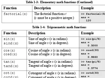
Some commonly used elementary MATLAB mathematical built-in functions are given in Tables 1-3 through 1-5. A complete list of functions organized by cat-egory can be found in the Help Window.

Tutorial 1-2: Using the sqrt built-in function.

>> sqrt(64) ans =

8

>> sqrt(50+14*3) ans =

9.5917

>> sqrt(54+9*sqrt(100)) ans =

12

>> (15+600/4)/sqrt(121) ans =

15 >>

Table 1-3: Elementary math functions

Function Description Example

sqrt(x) Square root. >> sqrt(81)

ans = 9

nthroot(x,n) Real nth root of a real number x. (If x is negative n must be an odd integer.)

>> nthroot(80,5) ans =

2.4022

exp(x) Exponential . >> exp(5)

ans = 148.4132

abs(x) Absolute value. >> abs(-24)

ans = 24

log(x) Natural logarithm.

Base e logarithm (ln).

>> log(1000) ans =

6.9078

log10(x) Base 10 logarithm. >> log10(1000)

ans = 3.0000

Argument is a number.

Argument is an expression.

Argument includes a function.

Function is included in an expression.

ex

(27)

1.5 Elementary Math Built-in Functions

15

The inverse trigonometric functions are asin(x), acos(x), atan(x), acot(x) for the angle in radians; and asind(x), acosd(x), atand(x), acotd(x) for the angle in degrees. The hyperbolic trigonometric functions are sinh(x), cosh(x), tanh(x), and coth(x). Table 1-4 uses pi, which is equal to π (see Section 1.6.3).

factorial(x) The factorial function x!

(x must be a positive integer.)

>> factorial(5) ans =

120

Table 1-4: Trigonometric math functions

Table 1-5: Rounding functions

round(x) Round to the nearest integer. >> round(17/5)

ans = 3

fix(x) Round toward zero. >> fix(13/5)

ans = 2

ceil(x) Round toward infinity. >> ceil(11/5)

ans = 3

floor(x) Round toward minus infinity. >> floor(-9/4)

ans = -3

rem(x,y) Returns the remainder after x is

divided by y.

>> rem(13,5) ans =

3 Table 1-3: Elementary math functions (Continued)

(28)

1.6 D

EFINING

S

CALAR

V

ARIABLES

A variable is a name made of a letter or a combination of several letters (and dig-its) that is assigned a numerical value. Once a variable is assigned a numerical value, it can be used in mathematical expressions, in functions, and in any MAT-LAB statements and commands. A variable is actually a name of a memory loca-tion. When a new variable is defined, MATLAB allocates an appropriate memory space where the variable’s assignment is stored. When the variable is used the stored data is used. If the variable is assigned a new value the content of the memory location is replaced. (In Chapter 1 we consider only variables that are assigned numerical values that are scalars. Assigning and addressing variables that are arrays is discussed in Chapter 2.)

1.6.1 The Assignment Operator

In MATLAB the = sign is called the assignment operator. The assignment opera-tor assigns a value to a variable.

• The left-hand side of the assignment operator can include only one variable name. The right-hand side can be a number, or a computable expression that can include numbers and/or variables that were previously assigned numerical values. When

the Enter key is pressed the numerical value of the right-hand side is assigned to

the variable, and MATLAB displays the variable and its assigned value in the next two lines.

The following shows how the assignment operator works.

sign(x) Signum function. Returns 1 if

, –1 if , and 0 if .

>> sign(5) ans =

1

>> x=15 x = 15

>> x=3*x-12 x =

33 >>

Table 1-5: Rounding functions (Continued)

x>0 x<0

x = 0

Variable_name = A numerical value, or a computable expression

The number 15 is assigned to the variable x.

MATLAB displays the variable and its assigned value.

(29)

1.6 Defining Scalar Variables

17

The last statement ( ) illustrates the difference between the assignment operator and the equal sign. If in this statement the = sign meant equal, the value of x would be 6 (solving the equation for x).

The use of previously defined variables to define a new variable is demon-strated next.

• If a semicolon is typed at the end of the command, then when the Enter key is pressed, MATLAB does not display the variable with its assigned value (the vari-able still exists and is stored in memory).

• If a variable already exists, typing the variable’s name and pressing the Enter key will display the variable and its value in the next two lines.

As an example, the last demonstration is repeated below using semicolons.

• Several assignments can be typed in the same line. The assignments must be sepa-rated with a comma (spaces can be added after the comma). When the Enter key is pressed, the assignments are executed from left to right and the variables and their assignments are displayed. A variable is not displayed if a semicolon is typed instead of a comma. For example, the assignments of the variables a, B, and C above can all be done in the same line.

>> a=12 a = 12 >> B=4 B = 4

>> C=(a-B)+40-a/B*10 C =

18

>> a=12; >> B=4;

>> C=(a-B)+40-a/B*10; >> C

C = 18

>> a=12, B=4; C=(a-B)+40-a/B*10 a =

12 C = 18

x = 3x–12

Assign 12 to a.

Assign 4 to B.

Assign the value of the expres-sion on the right-hand side to the variable C.

The variables a, B, and C are defined but are not displayed since a semicolon is typed at the end of each statement.

The value of the variable C is displayed by typing the name of the variable.

(30)

• A variable that already exists can be reassigned a new value. For example:

• Once a variable is defined it can be used as an argument in functions. For exam-ple:

1.6.2 Rules About Variable Names

A variable can be named according to the following rules:

• Must begin with a letter.

• Can be up to 63 characters long.

• Can contain letters, digits, and the underscore character.

• Cannot contain punctuation characters (e.g., period, comma, semicolon).

• MATLAB is case sensitive: it distinguishes between uppercase and lowercase let-ters. For example, AA, Aa, aA, and aa are the names of four different variables.

• No spaces are allowed between characters (use the underscore where a space is desired).

• Avoid using the name of a built-in function for a variable (i.e., avoid using cos, sin, exp, sqrt, etc.). Once a function name is used to define a variable, the function cannot be used.

1.6.3 Predefined Variables and Keywords

There are 20 words, called keywords, that are reserved by MATLAB for various purposes and cannot be used as variable names. These words are:

break case catch classdef continue else elseif end for function global if otherwise parfor persistent return spmd switch try while

>> ABB=72; >> ABB=9; >> ABB ABB = 9 >>

>> x=0.75;

>> E=sin(x)^2+cos(x)^2 E =

1 >>

A value of 72 is assigned to the variable ABB.

A new value of 9 is assigned to the variable ABB.

(31)

1.7 Useful Commands for Managing Variables

19

When typed, these words appear in blue. An error message is displayed if the user tries to use a keyword as a variable name. (The keywords can be displayed by typ-ing the command iskeyword.)

A number of frequently used variables are already defined when MATLAB is started. Some of the predefined variables are:

ans A variable that has the value of the last expression that was not assigned to a specific variable (see Tutorial 1-1). If the user does not assign the value of an expression to a variable, MATLAB automatically stores the result in ans.

pi The number π.

eps The smallest difference between two numbers. Equal to 2^(–52), which is approximately 2.2204e–016.

inf Used for infinity.

i Defined as , which is: 0 + 1.0000i.

j Same as i.

NaN Stands for Not-a-Number. Used when MATLAB cannot determine a valid

numeric value. Example: 0/0.

The predefined variables can be redefined to have any other value. The vari-ables pi, eps, and inf, are usually not redefined since they are frequently used in many applications. Other predefined variables, such as i and j, are sometime redefined (commonly in association with loops) when complex numbers are not involved in the application.

1.7 U

SEFUL

C

OMMANDSFOR

M

ANAGING

V

ARIABLES

The following are commands that can be used to eliminate variables or to obtain information about variables that have been created. When these commands are typed in the Command Window and the Enter key is pressed, either they provide information, or they perform a task as specified below.

Command Outcome

clear Removes all variables from the memory.

clear x y z Removes only variables x, y, and z from the

memory.

who Displays a list of the variables currently in the

memory.

whos Displays a list of the variables currently in the

memory and their sizes together with informa-tion about their bytes and class (see Secinforma-tion 4.1).

1

(32)

1.8 S

CRIPT

F

ILES

So far all the commands were typed in the Command Window and were executed

when the Enter key was pressed. Although every MATLAB command can be

executed in this way, using the Command Window to execute a series of com-mands—especially if they are related to each other (a program)—is not conve-nient and may be difficult or even impossible. The commands in the Command Window cannot be saved and executed again. In addition, the Command Window is not interactive. This means that every time the Enter key is pressed only the last command is executed, and everything executed before is unchanged. If a change or a correction is needed in a command that was previously executed and the results of this command are used in commands that follow, all the commands have to be entered and executed again.

A different (better) way of executing commands with MATLAB is first to create a file with a list of commands (program), save it, and then run (execute) the file. When the file runs, the commands it contains are executed in the order that they are listed. If needed, the commands in the file can be corrected or changed and the file can be saved and run again. Files that are used for this purpose are called script files.

IMPORTANT NOTE: This section covers only the minimum that is

required in order to run simple programs. This will allow the student to use script files when practicing the material that is presented in this and the next two chapters (instead of typing repeatedly in the Command Window). Script files are considered again in Chapter 4 where many additional topics that are essential for understanding MATLAB and writing programs in script file are covered.

1.8.1 Notes About Script Files

• A script file is a sequence of MATLAB commands, also called a program.

• When a script file runs (is executed), MATLAB executes the commands in the order they are written just as if they were typed in the Command Window.

• When a script file has a command that generates an output (e.g., assignment of a value to a variable without a semicolon at the end), the output is displayed in the Command Window.

• Using a script file is convenient because it can be edited (corrected or other-wise changed) and executed many times.

• Script files can be typed and edited in any text editor and then pasted into the MATLAB editor.

(33)

1.8 Script Files

21 1.8.2 Creating and Saving a Script File

In MATLAB script files are created and edited in the Editor/Debugger Window. This window is opened from the Command Window. In the File menu, select

New, and then select Script. An open Editor/Debugger Window is shown in Fig-ure 1-6.

Once the window is open, the commands of the script file are typed line by line. MATLAB automatically numbers a new line every time the Enter key is pressed. The commands can also be typed in any text editor or word processor program and then copied and pasted in the Editor/Debugger Window. An example of a short program typed in the Editor/Debugger Window is shown in Figure 1-7. The first few lines in a script file are typically comments (which are not executed since the first character in the line is %) that describe the program written in the script file.

Figure 1-6: The Editor/Debugger Window.

Figure 1-7: A program typed in the Editor/Debugger Window.

The commands in the script file are typed line by line. The lines are num-bered automatically. A new line starts when the Enter key is pressed. Line

number

Comments. Define three

variables.

Calculating the two roots.

(34)

Before a script file can be executed it has to be saved. This is done by choosing Save As... from the File menu, selecting a location (many students save to a flash drive, which appears in the directory as Drive(F:) or (G:)), and entering a name for the file. When saved, MATLAB adds the extension .m to the name. The rules for naming a script file follow the rules of naming a variable (must begin with a letter, can include digits and underscore, no spaces, and up to 63 characters long). The names of user-defined variables, predefined variables, and MATLAB commands or functions should not be used as names of script files.

1.8.3 Running (Executing) a Script File

A script file can be executed either directly from the Editor Window by clicking on the Run icon (see Figure 1-7) or by typing the file name in the Command Win-dow and then pressing the Enter key. For a file to be executed, MATLAB needs to know where the file is saved. The file will be executed if the folder where the file is saved is the current folder of MATLAB or if the folder is listed in the search path, as explained next.

1.8.4 Current Folder

The current folder is shown in the “Current Folder” field in the desktop toolbar of the Command Window, as shown in Figure 1-8. If an attempt is made to execute a script file by clicking on the Run icon (in the Editor Window) when the current folder is not the folder where the script file is saved, then the prompt shown in

Figure 1-9 will open. The user can then change the current folder to the folder where the script file is saved, or add it to the search path. Once two or more differ-ent currdiffer-ent folders are used in a session, it is possible to switch from one to another in the Current Folder field in the Command Window. The current folder can also be changed in the Current Folder Window, shown in Figure 1-10, which can be opened from the Desktop menu. The Current Folder can be changed by choosing the drive and folder where the file is saved.

Figure 1-8: The Current folder field in the Command Window.

(35)

1.8 Script Files

23

An alternative simple way to change the current folder is to use the cd com-mand in the Comcom-mand Window. To change the current folder to a different drive, type cd, space, and then the name of the directory followed by a colon : and press

the Enter key. For example, to change the current folder to drive F (e.g., the flash

drive) type cd F:. If the script file is saved in a folder within a drive, the path to that folder has to be specified. This is done by typing the path as a string in the cd

command. For example, cd('F:\Chapter 1') sets the path to the folder

Chapter 1 in drive F. The following example shows how the current folder is changed to be drive E. Then the script file from Figure 1-7, which was saved in drive E as ProgramExample.m, is executed by typing the name of the file and pressing the Enter key.

Figure 1-9: Changing the current directory.

Figure 1-10: The Current Folder Window.

>> cd E:

>> ProgramExample x1 =

3.5000 x2 =

-1.2500

Current folder shown here.

Click here to change the folder.

Click here to browse for a folder.

Click here to go up one level in the file system.

The current directory is changed to drive E.

The script file is executed by typing the name of the file and pressing the Enter key.

(36)

1.9 E

XAMPLESOF

MATLAB A

PPLICATIONS

Sample Problem 1-1: Trigonometric identity

A trigonometric identity is given by:

Verify that the identity is correct by calculating each side of the equation, substi-tuting .

Solution

The problem is solved by typing the following commands in the Command Win-dow.

Sample Problem 1-2: Geometry and trigonometry

Four circles are placed as shown in the figure. At each point where two circles are in contact they are tangent to each other. Determine the distance between the centers C₂ and C₄. The radii of the circles are:

mm, mm, mm, and

mm.

Solution

The lines that connect the centers of the cir-cles create four triangles. In two of the trian-gles, ΔC1C2C3 and ΔC1C3C4, the lengths of all the sides are known. This information is used to calculate the angles γ₁ and γ₂ in these triangles by using the law of cosines. For example, γ1 is cal-culated from:

>> x=pi/5;

>> LHS=cos(x/2)^2 LHS =

0.9045

>> RHS=(tan(x)+sin(x))/(2*tan(x)) RHS =

0.9045

x

2

---cos2 tanx+sinx 2tanx

---=

x π

5

---=

Define x. Calculate the left-hand side.

Calculate the right-hand side.

R₁ = 16 R₂ = 6.5 R₃ = 12

(37)

1.9 Examples of MATLAB Applications

25

Next, the length of the side C2C4 is calculated by considering the triangle

ΔC1C2C4. This is done, again, by using the law of cosines (the lengths C1C2 and

C₁C₄ are known and the angle γ₃ is the sum of the angles γ₁ and γ₂).

The problem is solved by writing the following program in a script file:

When the script file is executed, the following (the value of the variable C2C4) is displayed in the Command Window:

Sample Problem 1-3: Heat transfer

An object with an initial temperature of that is placed at time t = 0 inside a chamber that has a constant temperature of will experience a temperature change according to the equation

where T is the temperature of the object at time t, and k is a constant. A soda can at a temperature of F (after being left in the car) is placed inside a refrigerator where the temperature is F. Determine, to the nearest degree, the temperature of the can after three hours. Assume k = 0.45. First define all of the variables and then calculate the temperature using one MATLAB command.

Solution

The problem is solved by typing the following commands in the Command Win-dow.

% Solution of Sample Problem 1-2

R1=16; R2=6.5; R3=12; R4=9.5;

C1C2=R1+R2; C1C3=R1+R3; C1C4=R1+R4; lengths of the sides.

Calculate γ₁, γ₂, and γ₃.

(38)

Sample Problem 1-4: Compounded interest

The balance B of a savings account after t years when a principal P is invested at an annual interest rate r and the interest is compounded n times a year is given by:

(1)

If the interest is compounded yearly, the balance is given by:

(2)

Suppose $5,000 is invested for 17 years in one account where the interest is com-pounded yearly. In addition, $5,000 is invested in a second account in which the interest is compounded monthly. In both accounts the interest rate is 8.5%. Use MATLAB to determine how long (in years and months) it would take for the bal-ance in the second account to be the same as the balbal-ance of the first account after 17 years.

Solution

Follow these steps:

(a) Calculate B for $5,000 invested in a yearly compounded interest account after 17 years using Equation (2).

(b) Calculate t for the B calculated in part (a), from the monthly compounded interest formula, Equation (1).

(c) Determine the number of years and months that correspond to t.

The problem is solved by writing the following program in a script file:

>> Ts=38; T0=120; k=0.45; t=3;

>> T=round(Ts+(T0-Ts)*exp(-k*t))

T = 59

% Solution of Sample Problem 1-4 P=5000; r=0.085; ta=17; n=12; B=P*(1+r)^ta

t=log(B/P)/(n*log(1+r/n))

years=fix(t)

months=ceil((t-years)*12)

Round to the nearest integer.

B P 1 r

n

---+

⎝ ⎠

⎛ ⎞nt

=

B ₌ P(1+r)t

Step (a): Calculate B from Eq. (2).

Step (b): Solve Eq. (1) for t, and calculate t.

Step (c): Determine the number of years.

(39)

1.10 Problems

27

When the script file is executed, the following (the values of the variables B, t, years, and months) is displayed in the Command Window:

1.10 P

ROBLEMS

The following problems can be solved by writing commands in the Command Window, or by writing a program in a script file and then executing the file.

1. Calculate:

>> format short g B =

years, and months are displayed

(40)

5. Calculate:

(a) Determine the radius of a sphere that has the same surface area as the cube.

(b) Determine the radius of a sphere that has the same volume as the cube.

11. The perimeter P of an ellipse with semi-minor axes a and

b is given approximately by: .

(a) Determine the perimeter of an ellipse with in. and in.

(b) An ellipse with has a perimeter of cm. Determine a and b.

12. Two trigonometric identities are given by:

(a) (b)

For each part, verify that the identity is correct by calculating the values of the left and right sides of the equation, substituting .

(41)

1.10 Problems

29

13. Two trigonometric identities are given by:

(a) (b)

For each part, verify that the identity is correct by calculating the values of the left and right sides of the equation, substituting .

14. Define two variables: alpha = 5π/8, and beta = π/8. Using these variables, show that the following trigonometric identity is correct by calculating the values of the left and right sides of the equation.

15. Given: . Use MATLAB to calculate the following

definite integral: .

16. In the triangle shown cm, cm, and

cm. Define a, b, and c as variables, and then:

(a) Calculate the angle α (in degrees) by

substi-tuting the variables in the Law of Cosines.

(Law of Cosines: )

(b) Calculate the angles β and γ (in degrees) using the Law of Sines.

(c) Check that the sum of the angles is .

17. In the triangle shown in., in., and .

Define a, b, and γ as variables, and then:

(a) Calculate the length of c by substituting the variables in the Law of Cosines.

(Law of Cosines: )

(b) Calculate the angles α and β (in degrees) using the Law of Sines.

(c) Verify the Law of Tangents by substituting the results from part (b) into the right and left sides of the equation.

(Law of Tangents:

(42)

18. For the triangle shown, mm, mm, and mm. Define a, b, and c as variables, and then:

(a) Calculate the angle γ (in degrees) by substituting

the variables in the Law of Cosines.

(Law of Cosines: )

(b) Calculate the radius r of the circle inscribed in

the triangle using the formula .

(c) Calculate the radius r of the circle inscribed in the triangle using the

for-mula , where .

19. In the right triangle shown cm and cm.

Define a and c as variables, and then:

(a) Using the Pythagorean Theorem, calculate b by typing one line in the Command Window.

(b) Using b from part (a) and the acosd function, calculate the angle α in degrees by typing one line in the Command Window.

20. The distance d from a point to a plane is

given by:

Determine the distance of the point from the plane

. First define the variables A, B, C, D, x0, y0, and z0, and then calculate d. (Use the abs and sqrt functions.)

21. The arc length s of the parabolic segment BOC is given by:

Calculate the arc length of a parabola with in. and in.

(43)

1.10 Problems

31

23. The voltage difference between points a and b in the Wheatstone bridge circuit is:

Calculate the voltage difference when

volts, ohms, ohms,

ohms, and ohms.

24. The prices of an oak tree and a pine tree are $54.95 and $39.95, respectively. Assign the prices to variables named oak and pine, change the display format to bank, and calculate the following by typing one command:

(a) The total cost of 16 oak trees and 20 pine trees. (b) The same as part (a), and add 6.25% sale tax.

(c) The same as part (b) and round the total cost to the nearest dollar.

25. The resonant frequency f (inHz) for the circuit shown is given by:

Calculate the resonant frequency when henrys, ohms, ohms, and farads.

26. The number of combinations of taking r objects out of n objects is given by:

A deck of poker cards has 52 different cards. Determine how many different combinations are possible for selecting 5 cards from the deck. (Use the built-in function factorial.)

27. The formula for changing the base of a logarithm is:

(44)

28. The current I (in amps) t seconds after closing the switch in the circuit shown is:

Given volts, ohms, and

henrys, calculate the current 0.003 seconds after the switch is closed.

29. Radioactive decay of carbon-14 is used for estimating the age of organic

material. The decay is modeled with the exponential function ,

where t is time, is the amount of material at , is the amount of material at time t, and k is a constant. Carbon-14 has a half-life of approxi-mately 5,730 years. A sample of paper taken from the Dead Sea Scrolls shows that 78.8% of the initial ( ) carbon-14 is present. Determine the esti-mated age of the scrolls. Solve the problem by writing a program in a script file. The program first determines the constant k, then calculates t for

, and finally rounds the answer to the nearest year.

30. Fractions can be added by using the smallest common denominator. For example, the smallest common denominator of 1/4 and 1/10 is 20. Use the MATLAB Help Window to find a MATLAB built-in function that determines the least common multiple of two numbers. Then use the function to show that the least common multiple of:

(a) 6 and 26 is 78. (b) 6 and 34 is 102.

31. The Moment Magnitude Scale (MMS), denoted , which is used to

mea-sure the size of an earthquake, is given by:

where is the magnitude of the seismic moment in dyne-cm (measure of the energy released during an earthquake). Determine how many times more

energy was released from the earthquake in Sumatra, Indonesia ( ),

in 2007 than the earthquake in San Francisco, California ( ), in 1906.

32. According to special relativity, a rod of length L moving at velocity v will shorten by an amount , given by:

where c is the speed of light (about m/s). Calculate how much a rod 2 meter long will contract when traveling at 5,000 m/s.

(45)

1.10 Problems

33

33. The monthly payment M of a loan amount P for y years and interest rate r can be calculated by the formula:

(a) Calculate the monthly payment of a $85,000 loan for 15 years and interest rate of 5.75% ( ). Define the variables P, r, and y and use them to calculate M.

(b) Calculate the total amount needed for paying back the loan.

34. The balance B of a savings account after t years when a principal P is invested at an annual interest rate r and the interest is compounded yearly is given by . If the interest is compounded continuously, the balance is

given by . An amount of $40,000 is invested for 20 years in an

account that pays 5.5% interest and the interest is compounded yearly. Use MATLAB to determine how many fewer days it will take to earn the same if the money is invested in an account where the interest is compounded contin-uously.

35. The temperature dependence of vapor pressure p can be estimated by the Anteing equation:

where ln is the natural logarithm, p is in mm Hg, T is in kelvins, and A, B, and C are material constants. For toluene (C₆H₅CH₃) in the temperature range

from 280 to 410 K the material constants are , , and

. Calculate the vapor pressure of toluene at 315 and 405 K.

36. Sound level in units of decibels (dB) is determined by:

where p is the sound pressure of the sound, and Pa is a

refer-ence sound pressure (the sound pressure when dB).

(a) The sound pressure of a passing car is Pa. Determine its sound level in decibels.

(46)

37. Use the Help Window to find a display format that displays the output as a ratio of integers. For example, the number 3.125 will be displayed as 25/8. Change the display to this format and execute the following operations:

(a) (b)

38. The steady-state heat conduction q from a cylin-drical solid wall is determined by:

where k is the thermal conductivity. Calculate q for a copper tube ( Watts/oC/m) of length

cm with an outer radius of cm

and an inner radius of cm. The external temperature is C and

the internal temperature is C.

39. Stirling's approximation for large factorials is given by:

Use the formula for calculating 20!. Compare the result with the true value obtained with MATLAB’s built-in function factorial by calculating the

error ( ).

40. A projectile is launched at an angle and speed of . The projectile’s travel time ,

maximum travel distance , and maximum

height are given by:

Error = (TrueVal–ApproxVal) ⁄ TrueVal

(47)

35

Chapter 2 Creating Arrays

The array is a fundamental form that MATLAB uses to store and manipulate data. An array is a list of numbers arranged in rows and/or columns. The simplest array (one-dimensional) is a row or a column of numbers. A more complex array (two-dimensional) is a collection of numbers arranged in rows and columns. One use of arrays is to store information and data, as in a table. In science and engineering, one-dimensional arrays frequently represent vectors, and two-dimensional arrays often represent matrices. This chapter shows how to create and address arrays, and Chapter 3 shows how to use arrays in mathematical operations. In addition to arrays made of numbers, arrays in MATLAB can also be a list of characters, which are called strings. Strings are discussed in Section 2.10.

2.1 C

REATINGA

O

NE

-D

IMENSIONAL

A

RRAY

(V

ECTOR

)

A one-dimensional array is a list of numbers arranged in a row or a column. One example is the representation of the position of a point in space in a three-dimen-sional Cartesian coordinate system. As shown in Figure 2-1, the position of point

A is defined by a list of the three numbers 2, 4, and 5, which are the coordinates of the point.

The position of point A can be expressed in terms of a position vector:

r_A = 2i + 4j +5k

where i, j, and k are unit vectors in the direction of the x, y, and z axes, respec-tively. The numbers 2, 4, and 5 can be used to define a row or a column vector.

Any list of numbers can be set up as a vector. For example, Table 2-1 con-tains population growth data that can be used to create two lists of numbers—one of the years and the other of the

popula-tion values. Each list can be entered as elements in a vector with the numbers placed in a row or in a column.

x

y z

A (2, 4, 5)

2 4

5