Chp03 – General Random Variables

Introduction to Probability

SECOND EDITION

Dimitri

P.

Bertsekas and John N. Tsitsiklis

Massachusetts Institute of Technology

WWW site for book information and orders

http://www.athenasc.com

3

General R andom Variable s

Contents

3 . 1 . Continuous Random Variables and PDFs 3.2. Cumulative Distribution Functions . . . 3.3. Normal Random Variables . . . . 3.4. Joint PDFs of Multiple Random Variables 3.5. Conditioning . . . .

3.6. The Continuous Bayes' Rule 3.7. Summary and Discussion

Problems . . . .

· p. 140 · p. 148 · p. 153 · p. 158 · p. 164 · p. 178 · p. 182 · p. 184

140

General Random Variables Chap. 3

Random variables with a continuous range of possible values are quite common;

the velocity of a vehicle traveling along the highway could be one example. If the

velocity is measured by a digital speedometer, we may view the speedometer's

reading as a discrete random variable. But if we wish to model the exact velocity,

a continuous random variable is called for. Models involving continuous random

variables can be useful for several reasons. Besides being finer-grained and pos­

sibly more accurate, they allow the use of powerful tools from calculus and often

admit an insightful analysis that would not be possible under a discrete model.

All of the concepts and methods introduced in Chapter 2, such as expec­

tation, PMFs, and conditioning, have continuous counterparts. Developing and

interpreting these counterparts is the subject of this chapter.

3.1

CONTINUOUS RANDOM VARIABLES AND PDFS

A random variable

X

is called

continuous

if there is a nonnegative function

f x,

called the

probability density function of

X ,

or PDF for short, such that

P(X

E

B)

₌

1

fx(x) dx,

for every subset

B

of the real line.

t

In particular, the probability that the value

of

X

falls within an interval is

P(a X

<

b)

₌

f.b

fx(x) dx,

and can be interpreted as the area under the graph of the PDF

(

see Fig.

3. 1 ) .

For any single value

a,

we have

P(X

=

a ) =

faa

fx{x) dx

=

O.

For this reason,

including or excluding the endpoints of an interval has no effect on its probability:

P(a � X � b) = P(a

<

X

<

b) = P (a

<

X

<

b)

=

P(a

<

X � b) .

Note that to qualify as a PDF, a function

fx

must be nonnegative, I.e. ,

fx(x)

;:::: 0

for every

x,

and must also have the normalization property

I:

fx{x)dx

= P(-oc

<

X

<

oc

)

=

1 .

3. 1

(

X

that X takes a value in an is the shaded area in

x

6]

(t)

· 8,

3.2: of the

mass per around x. If 6 is very

that X takes

x + 0] is which

is 6.

if 0 :::; X :::; 1 ,

P D F fxCr)

normalization property. Indeed, we have within

3. 1

so

rI •

• , I

'

3.4: A piecewise constant P D F _{involving three intervals.}

1

125

3

= P(rainy day

)

=

20

(x) =

125

C2

20

1 2

15 '

C2

=

- . a

constant form

=

{ ��!

if a, � x < ai+ l l i = I , 2 , . . . , n - I ,

a 1

)

a2 : ' - . ) an are some with at < ai+ 1 for all i, and

Cl, C2, ... ) Cn

are

constants

by as in

m ust be such that the normalization

n-l1ai+1

n - l

1 = (x) dx = Ci dx = ci (ai+ l - ad.

i= l ai i = l

!X (X) =

{

1

O .

if 0 < x ::; 1 ,

determined

a

becomes infinitely large as x approaches zero� this is still a valid

144 General Random Variables

The

expected value

or

expectation

or

mean

of a continuous random variable

X

is defined by

t

E[X] =

I:

xfx(x) dx.

This is similar to the discrete case except that the PMF is replaced by the PDF,

and summation is replaced by integration. As in Chapter

2. E[X]

can be inter­

preted as the " center of gravity" of the PDF and, also. as the anticipated average

value of

X

in a large number of independent repetitions of the experiment. Its

nite or undefined. More concretely. we will say that the expectation is well-defined if

f�x

Ixlix

(x) dx

< ce. In that case, it is known that the integral

f�Xi

xix

(x) dx

takes a finite and unambiguous value.

For an example where the expectation is not well-defined. consider a random variable

X

with PDF

ix(x)

=

c/(l

+

x2),

where

c

is a constant chosen to enforce the normalization condition. The expression

Ixlix

(x)

can be approximated by

c/lxl

when

Ixl

is large. Using the fact

fiX

(Ilx) dx

= x. one can show that

r::=x

Ixlix

(x) dx

= :)c . Thus. E[X] is left undefined. despite the symmetry of the PDF around zero.

Sec. 3. 1 Continuous Random Variables and PDFs 145

g(x)

=

1

for

x

>

O.

and

g(x)

=

O.

otherwise. Then Y

=

g(X)

is a discrete

random variable taking values in the finite set

{O. I}.

In either case. the mean

of

g(X)

satisfies the

expected value rule

E[g(X)]

=

I: g(x)fx(x) dx,

in complete analogy with the discrete case; see the end-of-chapter problems.

The

nth moment

of a continuous random variable

X

is defined as

E[xn] .

the expected value of the random variable

Xn.

The

variance.

denoted by

var

(

X

)

. is defined as the expected value of the random variable

(X - E[X]) 2.

We now summarize this discussion and list a number of additional facts

that are practically identical to their discrete counterparts.

Expectation of a Continuous Random Variable and its Properties

Let

X

be a continuous random variable with PDF

fx.

•

The expectation of

X

is defined by

E[X]

=

I: xfx(x) dx.

•

The expected value rule for a function

g(X)

has the form

E[g(X)]

=

I: g(x)fx(x) dx.

•

The variance of

X

is defined by

var

(

X

)

=

E [ (X - E[X])2]

=

i:

(x

- E[X]) 2

fx(x) dx.

•

We have

0 ::;

var

(

X

)

=

E[X2] - (E[X]) 2 .

•

If Y

=

aX

+

b, where

a

and b are given scalars, then

E[Y]

=

aE[X]

+

b,

var

(

Y

)

=

a2var

(

X

)

.

Example

3.4.

Mean and Variance of the Uniform Random Variable.

Consider

a

uniform

PDF

over an interval [a. b].

as

in Example

3. 1 .

\Ve have

jx

E[X]

= _

146

= !X2

1

b

b - a 2

a

1

b

2

- a2

-- .

---b - a

2

a + b

General Random Variables

as one expects based on the symmetry of the PDF around

_{(a + b)/2.}

Chap. 3

To obtain the variance, we first calculate the second moment. We have

E[X2]

=

l

b 2 dx =

__

1

l

b x2 dx

b - a

b - a

a a

Thus, the variance is obtained as

(a + b)

2

_

(b - a)

2

after some calculation.

Exponential Random Variable

4

-

12

An

exponential

random variable has a PDF of the form

{

Ae-AX

_if

x

> _°

fx(x)

=

_0,

'

_otherwi�e,

where

A

is a positive parameter characterizing the PDF

(

see Fig. 3.5). This is a

legitimate PDF because

100

fx(x) dx

=

Ae-AX

dx

=

_e_.xx

I

OO

=

1 .

-00

0

Note that the probability that

X

exceeds a certain value decreases exponentially.

Indeed, for any

a > 0,

we have

3. 1

J ... large A

3.5: The PDF of an random variable.

a

for the time being we will

analytically.

the

can

be

1

E[X]

=

�

_'

var(X )

= ,.\2 ' 1

can be verified by straightforward

E[X]

=

== 0

-1

- � .

as

we now

by

the second

IS

E[X2]

=

[10

=

(

Ax

)

I

:

+

100

2

=

0

-,.\ 2

148 General Random Variables

Finally, using the formula var(X)

=

E[X2] -

(

E[X]) 2 . we obtain

2 1 1

var(X)

=

_{,,\2 - ,,\2}

=

_{,,\2 '}

Chap. 3

Example

3.5. The time until a small meteorite first lands anywhere in the Sahara desert is modeled as an exponential random variable with a mean of

10

days. The time is currently midnight. What is the probability that a meteorite first lands

We have been dealing with discrete and continuous random variables in a some­

what different manner. using PMFs and PDFs, respectively. It would be desir­

able to describe all kinds of random variables with a single mathematical concept.

This is accomplished with the

cumulative distribution function,

or CDF for

short. The CDF of a random variable X is denoted by

F x

and provides the

probability P(X ::; x). In particular, for every

x

we have

if X is discrete,

Fx(x)

=

P(X

::; x)

=

if X is continuous.

Loosely speaking, the CDF

Fx(x)

" accumulates" probability "up to" the value

x.

Any random variable associated with a given probability model has a CDF,

regardless of whether it is discrete or continuous. This is because {X

::;

x}

is

always an event and therefore has a well-defined probability. In what follows, any

unambiguous specification of the pro babili ties of all events of the form {X

::;

.r},

be it through a PMF, PDF, or CDF. will be referred to as the

probability law

of the random variable X.

the formulA.

and has a staircase

mass . Note _that _{at t he} of _{the two}

1 b -a

2

1 . . . . . .

----variables. T he C D F 15 re l ated _to the

at t he

3 . 7: CDFs of some continuous random variables. The CDF is related to t he PDF the

<

Thus. t he PDF

x

can be obtained from the CDF

For a continuous random t he CDF has no

dt.

Le . . it is continuous.

150

General Random Variables Chap. 3

Properties of

a

CDF

The

CDF

Fx

of a random variable

X

is defined by

Fx(x)

= P(X

::; x),

for all

x,

and has the following properties.

•

F x

is monotonically nondecreasing:

if

x ::; y,

then

Fx(x)

<

Fx(y).

•

Fx(x)

tends to

0

as

x

- - 00

, and to

1

as

x

- 00.

•

If

X

is discrete, then

Fx(x)

is a piecewise constant function of

x.

•

If

X

is continuous, then

Fx(x)

is a continuous function of

x.

•

If

X

is discrete and takes integer values, the

PMF

and the

CDF

can

be obtained from each other by summing or differencing:

k

Fx(k)

=

L

px(i),

i=-oo

px(k)

=

P

(

X

::; k)

- P(X

::; k

- 1 ) =

Fx(k) - Fx(k

- 1 ) ,

for all integers

k.

•

If

X

is continuous, the

PDF

and the

CDF

can be obtained from each

other by integration or differentiation:

Fx(x)

=

[

X

oo

/x(t) dt,

/x(x)

=

dFx

dx (x).

(The second equality is valid for those

x

at which the

PDF

is contin­

uous.)

Sometimes, in order to calculate the

PMF

or

PDF

of a discrete or contin­

uous random variable. respectively. it is more convenient to first calculate the

CDF.

The systematic use of this approach for functions of continuous random

variables will be discussed in Section

4. 1 .

The following is a discrete example.

Sec. 3.2 Cumulative Distribution Functions

151

The preceding line of argument can be generalized to any number of random variables

Xl . . . Xn .

In particular, if the events

{Xl

�

x}

. . . . , {Xn

�

X}

are

Because the

CDF

is defined for any type of random variable, it provides a conve­

nient means for exploring the relations between continuous and discrete random

variables.

A

particularly interesting case in point is the relation between geo­

metric and exponential random variables.

1 52 3

x >

1

3.8: and the We

(n), n = 1 . 2 , . . . ,

where 6 is chosen so that e - '\ o = I - p . As 6 ra.ndom variable can be

two

1 -

_so

are

to or if it

1

-

---dx = 1

3 . 9 : A normal PDF and with IJ. = 1 and 1 . We observe that

the PDF is around its mean 11-, and has a characteristic bel l

As x further from 11 . t he term e - decreases very In this the PDF is very dose to zero outside the i nterval 1 , 3]

Inean can

e - dy

so Inean can

we

153

154 General Random Variables Chap. 3

The last equality above is obtained by using the fact

--

1

100

e-y2 /2

dy

= 1 ,

J27T

-00

which is just the normalization property of the normal PDF for the case where

Il =

0 and (j

=

1.

A

normal random variable has several special properties. The following

one is particularly important and will be justified in Section 4. 1.

Normality is Preserved by Linear Transformations

If X is a normal random variable with mean

Il

and variance (j2, and if a =f. 0,

b are scalars, then the random variable

Y

=

aX + b

is also normal, with mean and variance

E[Y]

=

all + b,

var(Y)

=

a2(j2.

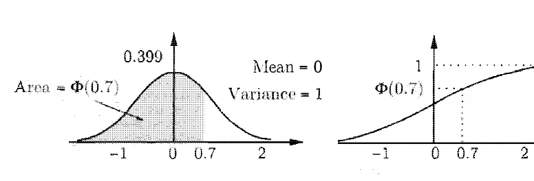
The Standard Normal Random Variable

A

normal random variable Y with zero mean and unit variance is said to be a

standard normal.

Its CDF is denoted by cI>:

1

1Y

2

cI>(y)

=

P

(Y ::; y)

=

P

(Y

<

y)

e-t

/2

dt.

It is recorded in a table (given in the next page), and is a very useful tool

for calculating various probabilities involving normal random variables; see also

Fig. 3.10.

Note that the table only provides the values of cI>(y) for y

�

0, because the

omitted values can be found using the symmetry of the PDF. For example, if Y

is a standard normal random variable, we have

cI>( -0.5)

=

P(Y

::; -0.5)

=

P(Y

�

0.5)

=

1 -

P(Y

<

0.5)

=

1 - cI>(0.5)

=

1 - .6915

=

0.3085.

More generally, we have

Sec. 3.3 Normal Random Variables 155

General Randolll Variables

by

y

₌

Y

is a it is normal.

- 1-1

- ₌

0,

var ( Y ) _{= =} 1 .

a

Thus,

Y

is a standard normal random variable. This

the probability of any event defined in of X : we

of and then use the standard nonnal table.

IvIean = 0

= 1

Figure 3 . 1 0 : The P DF

(y)

=

Chap. 3

of t he standard normal random variable. The n_{oted by <1>, is} recorded _{in a table.}

w h ich is

de-Example 3 . 7. Using the Normal Table. The annual snowfall at a particular location is modeled as a normal random with a mean of j.L = 60

a (J = is that

snowfall will be at least 80 i nches?

X snow accumulation, viewed as a normal random variable, and

y

= X - J1 =

(J

be the correspondi ng standard normal random variable. We have

P (X

>

80) = P

(X

- 60

>

80 - 60

)

=

- ₂₀ - ₂₀

(y

>

- 80 -₂₀ =

where 4> is the CDF of the standard normal. We read the value 4> ( 1) from the table:

Sec. 3.3 Normal Random Variables 157

so that

P(X � 80) = 1 - cIl(l) = 0.1587.

Generalizing the approach in the preceding example, we have the following

procedure.

CDF Calculation for a Normal Random Variable

For a normal random variable X with mean

Jl

and variance 0'2, we use a

two-step procedure.

(a

)

"Standardize" X, i.e., subtract

Jl

and divide by

a

to obtain a standard

normal random variable

Y.

(b

)

Read the CDF value from the standard normal table:

P(X S

x

)

=

P

(

X

/l

<

/l

)

=

P

(

y

<

x

u /l

)

= 1> /l

)

_.

Normal random variables are often used in signal processing and communi­

cations engineering to model noise and unpredictable distortions of signals. The

following is a typical example.

Example

3.8.

Signal Detection.

A binary message is transmitted as a signal s, which is either - l or + 1 . The communication channel corrupts the transmission with additive normal noise with mean J-L = 0 and variance a2• The receiver concludes that the signal - 1 (or + 1 ) was transmitted if the value received is < 0 (or � 0,

shaded

is transmitted .

3.8. The area of t he of er ror in the two cases w here _{- 1} and ₊ 1

3

number independent identically distributed (not necessarily normal) ran­

dom variables has an approximately normal cnp,

of the

cnp

of

the

theorem� which will be

d

is

cu

ss

ed

of a

PDF

to the

c

ase mult

i

ple random variables.

p

a

r

all

el the discrete case.

that two continuous random

are can be

we

uce j

o

i

n

t

,

i

nte

rp

r

e

t

atio

n

as

PDF

Jx.Y if fx.Y is a nonnegative function that satisfies

((X�

_Y)

E

(x,

y)

dx

saIne of a

joint

of

two-dimensional

that t he integration is

carried

o

v

er the

set B.

In t he

above Ineans case where

B is

a of ==

{ (x:

y) I

a

�

x

� b, c :::; y

::;

d},

we

d b

Sec. 3.4 Joint PDFs of Multiple Random Variables

159

Furthermore, by letting

B

be the entire two-dimensional plane, we obtain the

normalization property

1:1:

fx.y(x,y)dxdy

= 1 .

To interpret the joint PDF, we let

0

be a small positive number and consider

the probability of a small rectangle. We have

lc+61a+6

P(a < X < a+o, c ::;

Y

< c+o)

c a

fX'y(x,y)dxdy

�

fx.Y(a,c)·o2,

so we can view

fx,Y(a, c)

as

the "probability per unit area" in the vicinity of

(a. c).

_{The joint PD F contains all relevant probabilistic information on the random}

variables

X,

Y ,

and their dependencies. It allows us to calculate the probability

of any event that can be defined in terms of these two random variables. As

a special case, it can be used to calculate the probability of an event involving

only one of them. For example, let

A

be a subset of the real line and consider

the event

{X

E

A}.

We have

P(X

E

A)

=

p(X

E A

and

Y

E (-00,

(0))

=

i

I:

fx,Y(x, y) dydx.

Comparing with the formula

P(X

E

A)

=

i

fx(x) dx.

we see that the

marginal

PDF

fx

of

X

is given by

fx{x)

=

i:

fx.y(x, y) dy.

Similarly,

fy(y)

=

1:

fx,y{x, y) dx.

Example

3.9.

Two-Dimensional Uniform PDF.

Romeo and Juliet have a date at a given time, and each will arrive at the meeting place with a delay between

o and 1 hour (recall the example given in Section 1 .2). Let X and Y denote the delays of Romeo and Juliet, respectively. Assuming that no pairs (x. y) in the unit square are more likely than others, a natural model involves a joint PDF of the form

{ c.

if 0 S x S 1 and 0 S y S I ,

3

where

c

is a constant. this to

y)

=

I ,

we must have

c == 1 .

is an a us some

S of two-dimensional plane. The corresponding u niform joint PDF on S

is deft ned to be

{

area l

of S ! O.

any set A C

((X.

Y ) E

A)

=

J J

fx,y

_y) (:r· Y) E A

Y)

if

Y)

E

otherwise. in A is

area of

A

Example are told that t he jOint PDF of t he random variables X and

Y is a constant c on the set S 3. and is zero We wish to

Y .

fx.y (x, y) = c =

1 /4, for

y)

E marginal PDF f X (x) for SOIne particular X l we

(with respect to

y)

the joint PDF over the vertical. ]ine correspond ing to that x .

is We can

1 6 1 The needle will intersect the closest

162 General Random Variables

The probability of intersection can be empirically estimated, by repeating the ex­ periment a large number of times. Since it is equal to 2l/7rd, this provides us with a method for the experimental evaluation of 7r.

Joint CDFs

If

X

and Y are two random variables associated with the same experiment, we

define their joint CDF by

Fx,Y(x, y)

=

P(X �

X,

Y

< y).

As in the case of a single random variable, the advantage of working with the

CDF is that it applies equally well to discrete and continuous random variables.

In particular, if

X

and Y are described by a joint PDF

j X,Y,

then

Conversely, the PDF can be recovered from the CDF by differentiating:

Sec. 3.4 Joint PDFs of Multiple Random Variables 163

Expectation

If

X

and Y are jointly continuous random variables and

9

is some function, then

Z

=

g(X,

Y) is also a random variable. We will see in Section

4. 1

methods for

computing the PDF of

Z,

if it has one. For now, let us note that the expected

value rule is still applicable and

E[g(X,

Y)

]

=

I: I: g(x, y)fx,y(x, y) dxdy.

As an important special case, for any scalars

a,

b,

and

c,

we have

E[aX

+ b

Y

+

c

]

=

aE[X]

+ b

E

r

Y

l

+

c.

More than Two Random Variables

The joint PDF of three random variables

x,

Y , and

Z

is defined in analogy with

the case of two random variables. For example, we have

P((X,

Y, Z)

E

B)

=

j j jfx,y,z(x,y, z) dxdydz,

(x,y,z) E B

for any set

B.

We also have relations such as

and

fx,Y(x, y)

=

I: fx,Y,z(x, y, z) dz,

fx(x)

=

I: I: fx,Y.z(x, y, z) dydz.

The expected value rule takes the form

E[g(X,

Y,

Z)

]

=

I: I: I: g(x, y, z)fx.Y,z(x, y, z) dxdydz,

and if

9

is linear, of the form

aX

+ b

Y

+

cZ,

then

E[aX

+ b

Y

+

cZ

]

=

aE[X]

+ b

E

r

Y

l

+

cE

[

Z

]

.

Furthermore, there are obvious generalizations of the above to the case of more

than three random variables. For example, for any random variables

Xl, X2, .. . ,

164

General Random Variables Chap. 3

Summary of Facts about Joint PDFs

Let

X

and

Y

be jointly continuous random variables with joint PDF

/x,y.

•

The

joint PDF

is used to calculate probabilities:

p((X,

Y)

E

B)

=

J J

/x,y(x, y) dxdy.

(x,y)EB

•

The

marginal PDFs

of

X

and

Y

can be obtained from the joint PDF,

using the formulas

/x(x)

=

I:

/x.y(x, y) dy, /y(y)

=

i:

/x.y(x, y) dx.

•

The

joint CDF

is defined by

Fx,Y(x, y)

=

P(X ::; x,

Y

::; y),

and

determines the joint PDF through the formula

82FX Y

/x,y(x, y)

=

(x, y),

for every

(x, y)

at which the joint PDF is continuous.

•

A

function

g(X,

Y)

of

X

and

Y

defines a new random variable, and

E [g(X,

Y)]

=

I: 1:

g(x, Y)/X,y(x, y) dx dy.

If

9

is linear, of the form

aX

+

bY

+

c,

we have

E[aX

+

bY

+ c

]

=

aE[X]

+

bErYl

+

c.

•

The above have natural extensions to the case where more than two

random variables are involved.

3.5

CONDITIONING

Similar to the case of discrete random variables. we can condition a random

variable on an event or on another random variable, and define the concepts

of conditional PDF and conditional expectation. The various definitions and

formulas parallel the ones for the discrete case, and their interpretation is similar,

except for some subtleties that arise when we condition on an event of the form

Sec. 3.5 Conditioning 165

Conditioning a Random Variable on an Event

The

conditional PDF

of a continuous random variable

X,

given an event

A

with

P(A)

>

0, is defined as a nonnegative function

fXIA

that satisfies

P(X E B I A)

=

is

fXIA(X) dx,

for any subset

B

of the real line. In particular, by letting

B

be the entire real

line, we obtain the normalization property

so that

fXIA

is a legitimate PDF.

In the important special case where we condition on an event of the form

{X E A},

with

P(X E A)

>

0, the definition of conditional probabilities yields

P(X B I X A)

E

E

=

P(X E B, X

E

A)

P(X

E

A)

P(X E A)

By comparing with the earlier formula, we conclude that

{

fx(x)

fXI{XEA}(X)

=

_P(X

E

A)

.

0,

if

x

E A,

otherwise.

As in the discrete case, the conditional PDF is zero outside the conditioning set.

Within the conditioning set , the conditional PDF has exactly the same shape as

the unconditional one, except that it is scaled by the constant factor

l/P(X E A),

so that

fXI{XEA}

integrates to 1; see Fig.

3. 14.

Thus, the conditional PDF is

similar to an ordinary PDF, except that it refers to a new universe in which the

event

{X E A}

is known to have occurred.

Example

3.13.

The Exponential Random Variable is Memoryless.

The time T until a new light bulb burns out is an exponential random variable with parameter

_A.

Ariadne turns the light on, leaves the room, and when she returns, t time units later. finds that the light bulb is still on. which corresponds to the event

1 66

3.14: The unconditional PDF Ix and the cond itional PDF Ix

where A is the interval [a, b] . Note that within conditioning event _{I { X E A }}

retains the same shape as Ix ! except that it is scaled along the vertical axis.

3

where we have used the expression for the CDF of an exponential random variable

of X is

of the time

t

that elapsed between the lighting of the bulb and Ariadne's arrival.

is known as the

memorylessness property

of the exponential. Generally, if we

remaining time up to completion

operation started .

When variables are

Suppose, for

a similar notion are jointly

with joint probability event of the form := { (X!

y) ==

{

(x)

=

two provide one

0,

f x I y . If we condition on a

E

A } ,

we have

can

method for obtaining the

PDF

of a random variable

X

{X

E

A},

is

is not of terms of multiple random variables. finally

which conditional

Sec. 3.5 Conditioning

167

the sample space, then

n

!x (x)

=

L

P(Ai)!XIAi (x).

i=l

To

j

ustify this statement, we use the total probability theorem from Chapter 1 ,

and obtain

11

P(X

�

_x

)

₌

L

P(AdP(X

�

x I

Ai) .

i= l

This formula can be rewritten

as

j

- oc

x

!X (t) dt

=

�

n

P(Ad

j.e

- oc

!XIA, (t) dt.

We then take the derivative of both sides, with respect to

x,

and obtain the

desired result.

Conditional

PDF

Given an Event

•

The conditional PDF

!XIA

of a continuous random variable

X,

given

an event

A

with

P(A)

>

0, satisfies

P(X

E

B I

A)

=

Is

!XIA(X) dx.

•

If

A

is a subset of the real line with

P(X

E

A)

>

0, then

{

!x (x)

_'f

_E

_A

!XI{XEA} (x)

=

P(X

E

A)

'

1 X ,

0,

otherwise.

•

Let

A I , A2, . . . ,An

be dis

j

oint events that form a partition of the sam­

ple space, and assume that

P(Ai)

>

0 for all

i,

_Then,

n

!X {x)

=

L

P(Ai)!xIA; (X)

i=l

(

a version of the total probability theorem

)

,

General Variables 3

Example 14. The metro train arrives at the station near your home every

at 6:00 a. m .

3 . 1 5 : The PDFs _. jYjA ' jYI B l and

your

X

l is a

5 y

lJ

in _{3. 1 4 .}

over the i nterval from 7: 1 0 to 7:30; see F ig. 3. 1 5 (a) . Let

events fy

a

A

= { 7: 1 0 � X � 7: = { yon board t he 7:

train}\

=

{7: 1 5 < ::; 7:30} = {you board t he 7:30

event your is 7:

to 7: 1 5. In t his case: time Y is also uniform and takes between

o and 5 minutes; see Fig. 3. 15(b) . Similarly, conditioned on B� Y is uniform and

o see 3. 1 5(c) . is

using the total probability

and is shown i n

(y)

=

3. 1 5(d) . _We

1 1 3 1 1

(y) _{= 4} .

_5"

_{+ "4}

.

15

= 10 !

1 3 1 1

(y)

= 4

· 0 +

4:

. 15 = - )

for 0 � y �

x 3. 15.

Example

1

=

is not

1

Y

I

y) == =

a

if

IYI �

T.

I Y IS

area of t

if + <

Sec. 3.5 Conditioning 171

To interpret the conditional PDF, let us fix some small positive numbers

(h

and

82,

and condition on the event

B =

{y

::;

Y

::;

y

+

82}.

We have

where

82

decreases to zero and write

P(x

< X <

x

+

81

I

Y

=

y)

�

fxlY(x

I

y)81, (81

small) ,

and, more generally,

P

(X

E

A I

Y

=

y)

=

i

f x IY (x

I

y) dx.

Conditional probabilities, given the zero probability event

{Y

=

y},

were left

undefined in Chapter

1 .

But the above formula provides a natural way of defining

such conditional probabilities in the present context. In addition, it allows us to

view the conditional PDF

fxlY(x

I

y)

(as a function of

x)

as a description of the

probability law of

X,

given that the event

{Y

=

y}

has occurred.

As in the discrete case, the conditional PDF

fxlY'

together with the

marginal PDF

fy

are sometimes used to calculate the joint PDF. Furthermore,

this approach can also be used for modeling: instead of directly specifying

fx,Y,

it is often natural to provide a probability law for Y, in terms of a PDF

fy,

and then provide a conditional PDF

fxlY(x

I

y)

for

X,

given any possible value

y

of Y.

172 General Random Variables Chap. 3

Conditional PDF Given a Random Variable

Let

X

and

Y

be jointly continuous random variables with joint PDF

fx,Y'

•

The joint, marginal, and conditional PDFs are related to each other

by the formulas

fx,Y(x, y)

=

fy(y)fxlY(x

I

y),

fx(x)

=

[:

fy(y)fxlY(x

I

y) dy.

The conditional PDF

fxlY(x

I

y)

is defined only for those

y

for which

fy(y)

> 0 .

•

We have

P(X

E

A I Y

₌

y)

=

L

fxlY(X

I

y) dx.

For the case of more than two random variables, there are natural exten­

sions to the above. For example, we can define conditional PDFs by formulas

such as

fx,Y.z(x, y, z)

fX,Ylz(x.y

I

z)

=

_{fz(z) .}

fx,Y.z(x, y. z)

fxlY,z(x

I

y, z)

=

f ( )

_{Y,Z y, z}

.

There is also an analog of the multiplication rule,

if

fz(z)

> 0,

if

fy,z(y, z)

> O.

fx.y.z(x. y. z)

=

fxlY,z(x

I

y. z)fYlz(Y

I

z)fz(z),

and of other formulas developed in this section.

Conditional Expectation

For a continuous random variable

X,

we define its

conditional expectation

Sec. 3. 5 Conditioning

173

Summary of Facts About Conditional Expectations

Let

X

snd

Y

be jointly continuous random variables, and let

A

be an event

with

P(A)

>

O.

•

Definitions:

The conditional expectation of

X

given the event

A

is

defined by

E[X

I

A]

=

I:

XJXIA (X) dx.

The conditional expectation of

X

given that

Y

=

y

is defined by

E[X

I

Y

=

y]

=

I:

_{xJx IY (x}

I

y) dx.

•

The expected value rule:

For a function

g(X),

we have

E[g(X)

I

A]

=

I:

g(X)JXIA (X) dx,

and

E[g(X)

I

Y

=

Y]

=

I:

g(x)JxlY (X

I

y) dx.

•

Total expectation theorem:

Let

AI, A2, .. . ,An

be disjoint events

that form a partition of the sample space, and assume that

P(Ad

>

0

for all

i.

Then,

n

E[X]

=

L

P(AdE[X I Ai].

i=l

Similarly,

E[X]

=

I:

E[X

I

Y

=

y]Jy (y) dy.

•

There are natural analogs for the case of functions of several random

variables. For example,

E[g(X,

Y)

I

Y

=

y]

=

J

g(x, y)JxlY (X

I

y) dx,

and

E[g(X,

Y)]

=

!

_E

[

g

_(X

,

Y)

I

Y

=

ylJy (y) dy.

114 General Random Variables

theorem, we start with the total probability theorem

n

fx(x) =

L

P(Ai)fxIAi (x),

i=l

multiply both sides by

x,

and then integrate from

- 00

to

00 .

Chap. 3

To justify the second version of the total expectation theorem, we observe

that

I:

E[X

I Y

=

y]fy(y) dy

=

I: [I:

xfxlY(x

I

y) dX

]

fy(y) dy

=

I: I:

xfxlY(x

I

y)fy(y) dxdy

=

I: I:

_{xfx,Y(x,y) dxdy}

=

L:

x

[L:

fx,Y(X,Y)dY

]

dx

=

I:

xfx(x) dx

= E[X].

The total expectation theorem can often facilitate the calculation of the

mean, variance, and other moments of a random variable, using a divide-and­

conquer approach.

Example

3.11.

Mean and Variance of a Piecewise Constant PDF.

Suppose that the random variable

X

has the piecewise constant PDF

{

1/3, if 0 � x � 1 , Ix {x) = 2/3, if 1 < x � 2,

0, otherwise,

(

see Fig. 3. 18). Consider the events

Al

₌

{X

lies in the first interval [0,

In,

A2

₌

{X

lies in the second interval

{

I

, 2]

} .

We have from the given PDF,

11

1

P{AI)

=

₀

_Ix

(x) dx

= 3'

_P{A2)

=

1

2

2

1

Ix

(x) dx

= 3·

now

use

=

1

l Ad

=

2 '

] :;

�,

J +

+

.r

2

y

PDF _for

mean a

moment

is

1 1 2 3 7

_ . _ + _ . - =::-

_{3 2 3 2 6 '}

1 1 2 7

= - . - + - . _ = -

_{3 3 3 3}

_{9 .}

1 1

, we see

x

y)

=

=

are two axes are

o

constant .

3

> 0

all

z .

Le. , sets

contours are described

3 . 1 9 : Contou rs of _the PDF of two

Sec. 3.5 Conditioning 177

If

X

and Y are independent, then any two events of the form

{X

E

A}

and

{

Y

E

B}

are independent. Indeed,

P(X

E

A

and Y

E

B)

=

1

fx.Y(x, y) dydx

yEB

=

1 1

_{xEA yEB}

fx(x)fy(y) dydx

=

1

fx(x) dx

1

fy(y) dy

xEA yEB

=

P(X

E

A)

P

(

Y

E

B).

In particular, independence implies that

Fx,Y(x. y)

=

P(X

_::;

x,

_{Y ::;}

y)

=

P(X

_::;

x)

P(Y

_::;

y)

=

Fx(x)Fy(y).

The converse of these statements is also true: see the end-of-chapter problems.

The property

Fx.y(x. y)

=

Fx(x)Fy(y).

for all

x. y.

can be used to provide a general definition of independence between two random

variables. e.g., if

X

is discrete and Y is continuous.

An argument similar to the discrete case shows that if

X

and Y are inde­

pendent, then

E [g(X)h(Y)]

=

E [g(X)] E [h(Y)] .

for any two functions

9

and

h.

Finally. the variance of the sum of

independent

random variables is equal to the sum of their variances.

Independence of Continuous Random Variables

Let

X

and Y be jointly continuous random variables.

•

X

and Y are

independent

if

!x,Y(x, y)

=

!x(x)fy(y),

for all

x, y .

•

If

X

and Y are independent, then

1 78 3

for

g

the

g(X)

and h ( Y ) are independent , and we have

[g(X)h(Y)]

=

[g(X)] [h(Y)] .

• Y are

+ Y ) = var ( X ) ₊ var(Y ) .

3.6 THE

In many situations� we represent an unobserved phenomenon by a random able X with

PDF f

_x and we make a noisy measurement Y , which is modeled

in a conditional !y!x . Once value Y is

information does it prov ide on the unknown value of This setting is similar

1 . 4, where we rule it to

see The only we are now dealing w ith continuous random

x

Schematic d_escription of the inference problem

.

We have an random variable X with known and we obt ain a measurement

Y accordi ng to a cond i tio n al PDF _{!YIX '} Given an observed value y of Y 1 the i n ference problem is to evaluate the co_ndit_io_nal _PDF fX I Y (x I y) .

tured by the

From the formulas f X

Iy

pression is

!XIY

information i s provided { Y

= y} is

! X I Y I y) . It to evaluate this

=

Ix.y

=

Iy

j Y , it follows that

I

x

)

IY

I y) =

!XI Y I y) dx =

1 , an

I y)

=

.

icc

f _{X (t)!YIX (y I t) dt}

ex-Sec. 3.6 The Continuous Bayes ' Rule 179

Example

3.19. A light bulb produced by the General Illumination Company is known to have an exponentially distributed lifetime

_Y.

However, the company has been experiencing quality control problems. On any given day, the parameter ). of the PDF of

Y

is actually a random variable, uniformly distributed in the interval [1 . 3/2] . We test a light bulb and record its lifetime. What can we say about the

The available information about A is captured by the conditional PDF

!AIY(). I y),

which using the continuous Bayes' rule, is given by

f

AIY

(). I ) =

_y

100

!A().)!YIA (y l ).)

= _3/22).e- >'Y _' - 00

!A(t)!YIA(y

I

t) dt

!.

2te-ty

dt

Inference about a Discrete Random Variable

3

for

1 < ). <

-.

- - 2

In some cases, the unobserved phenomenon is inherently discrete. For some

examples, consider a binary signal which is observed in the presence of normally

distributed noise, or a medical diagnosis that is made on the basis of continuous

measurements such as temperature and blood counts. In such cases, a somewhat

different version of Bayes' rule applies.

We first consider the case where the unobserved phenomenon is described in

terms of

an

event

A

whose occurrence is unknown. Let

P(A)

be the probability of

event

A.

Let Y be a continuous random variable, and assume that the conditional

PDFs

fYIA(Y)

and

fYIAc(y)

are known. We are interested in the conditional

180

possibilities for the unobserved phenomenon of interest. Let

PN

be the PMF

of

N.

Let also

Y

_{be a continuous random variable which, for any given value}

n

of

N,

is described by a conditional PDF

fYIN(Y

I

n).

The above formula becomes

P(N

=

n

_I

Y

=

y)

=

I

n).

The denominator can be evaluated using the following version of the total prob­

ability theorem:

so that

P(N

=

n

I Y

₌

y)

=

PN(n)fYIN(Y

I

n) .

LPN(i)fYIN(Y

I

i)

Example

3.20.

Signal Detection.

A binary signal

S

is transmitted, and we are given that

P(S

=

1 ) =

p

and

P(S

=

- 1 )

=

I -p.

The received signal is

Y

=

N

+

S

.

where N is normal noise, with zero mean and unit variance, independent of

S.

What is the probability that

S

= 1 , as a function of the observed value

y

of

Y?

Conditioned on

S

=

s, the random variable

Y

has a normal distribution with mean s and unit variance. Applying the formulas given above, we obtain

Sec. 3.6 The Continuous Bayes ' Rule 181

Inference Based on Discrete Observations

We finally note that our earlier formula expressing

P(A I Y = y)

in terms of

fYIA (y)

can be turned around to yield

Based on the normalization property

J�oc

fYIA(Y) dy =

1 .

an equivalent

expres-sion is

f ( ) - fy(y)P(A I Y = y)

YIA Y

- jOC

.

-oc

fy(t) P(A I Y = t) dt

This formula can be used to make an inference about a random variable

Y

when

an event

A

is observed. There is a similar formula for the case where the event

A

is of the form

{N = n},

where

N

is an observed discrete random variable that

depends on

Y

in a manner described by a conditional

PMF

PNly(n

I

y).

Bayes' Rule for Continuous Random Variables

Let

Y

be a continuous random variable.

•

If

X

is a continuous random variable, we have

and

fy(y)fxlY(x

I

y)

fx(x)fYlx(Y I x),

J

XIY x y

( I ) - fx(x)fYlx(Y lx)

-

_fy(y)

_

- 00

fx(x)fYlx(Y lx)

.

100

fx(t)fYlx(Y I t) dt

•

If

N

is a discrete random variable, we have

fy(y) P(N =

n

I

Y

= y) = pN(n)fYIN(Y In),

182 General Random Variables Chap. 3

Continuous random variables are characterized by PDFs, which are used to cal­

culate event probabilities. This is similar to the use of PMFs for the discrete case,

except that now we need to integrate instead of summing. Joint PDFs are similar

to joint Pl\lFs and are used to determine the probability of events that are de­

fined in terms of multiple random variables. Furthermore, conditional PDFs are

similar to conditional PMFs and are used to calculate conditional probabilities,

given the value of the conditioning random variable. An important application is

in problems of inference, using various forms of Bayes' rule that were developed

in this chapter.

There are several special continuous random variables which frequently

arise in probabilistic models. We introduced some of them, and derived their

mean and variance. A summary is provided in the table that follows.

Summary of Results for Special Random Variables

Continuous Uniform Over

[a, b]:

if

a �

x

< b,

0,

otherwise,

E

_[

X

]

= a + ₂ b ,

Exponential with Parameter

'x:

Sec. 3. 7 Summary and Discussion

Normal with Parameters 11 and

a2

> 0:

1 2 2

fx (x)

= e-(X-IL)

/20' ,

V"iia

E

[

X

]

=

11,

var

(

X

)

=

a2.

183

1 84 General Random Variables Chap. 3

P R O B L E M S

SECTION 3. 1 . Continuous Random Variables and PDFs

Problem 1. Let

X

be uniformly distributed in the unit interval [0, 1] . Consider the random variable

Y

=

g(X),

where

g(x)

=

{21.,

if _if

x

_{x >}

::; 1/3, _1/3.

Find the expected value of Y by first deriving its PMF. Verify the result using the expected value rule.

Problem 2. Laplace random variable. Let

X

have the PDF

f

x

( ) .A

x

= '2e

->'Ix l

,

where

.A

is a positive scalar. Verify that

f

x satisfies the normalization condition, and evaluate the mean and variance of

X.

Problem 3.

*

Show that the expected value of a discrete or continuous random vari­ able

X

satisfies

E[X]

=

J.x

P(X > x) dx

J.x

P(

X

<

-x) dx.

Solution. Suppose that

X

is continuous. We then have

where for the second equality we have reversed the order of integration by writing the set

{(x. y)

1 0 ::;

x

< oc.

x ::; y

< oc} as

{ (x. y)

1 0 ::;

x ::; y,

0 ::;

y

< oo } . Similarly. we can show that

Problems

Combining the two relations above, we obtain the desired result. If

X

is discrete, we have

P(X

>

_x)

=

IX>

LPX(Y)

o

y>x

=

L

(IV

P

x (y) dx

)

y>O 0

=

LPX(Y)(

III

dX

)

y>O 0

and the rest of the argument is similar to the continuous case.

Problem

4. * Establish the validity of the expected value rule

E

[

g(X)

]

=

I:

g(x)fx (x) dx,

where

X

is a continuous random variable with PDF

_{fx .}

185

Solution. Let us express the function 9 as the difference of two nonnegative functions,

where

g+ (x)

=

max{

g(x)

, O}, and

g- (x)

=

max{

-g(x),

O}. In particular. for any

t

2::: 0,

we have

_g(x)

>

t

if and only if

_{g+ (x)}

>

t.

We will use the result

E

[

g(X)

]

=

f.X>

p

(

g(X)

>

t

)

dt -

f.X>

_p

(

_g(X)

<

-t

)

dt

from the preceding problem. The first term in the right-hand side is equal to

100

fx (X) dX dt =

j

oo

fx (X) dt dx =

j

=

g+ (x)fx (x) dx.

o

I g(x» t } - 00 _{l 0:$ t<g(x)}}

- X>

By a symmetrical argument, the second term in the right-hand side is given by

f.=

p

(

g(X)

<

-t

)

dt

=

I:

g- (x)fx (x) dx.

Combining the above equalities, we obtain

186 General Random Variables Chap. 3

SECTION 3.2. Cumulative Distribution Functions

Problem

5.

Consider a triangle and a point chosen within the triangle according to the uniform probability law. Let

X

be the distance from the point to the base of the triangle. Given the height of the triangle, find the CDF and the PDF of

X.

Problem

6. Calamity Jane goes t o the bank to make a withdrawal, and i s equally likely to find 0 or

1

customers ahead of her. The service time of the customer ahead, if present, is exponentially distributed with parameter

>..

What is the CDF of Jane's waiting time?

(b) Calculate the CDF of the two-sided exponential random variable that h as PDF given by

Problem 9. * Mixed random variables.

Probabilistic models sometimes involve random variables that can be viewed as a mixture of a discrete random variable

Y

and a continuous random variable

Z.

By this we mean that the value of

X

is obtained according to the probability law of

Y

with a given probability

p.

and according to the probability law of

Z

with the complementary probability

1

-

p.

Then,

X

is called a

mixed random variable

and its CDF is given. using the total probability theorem, by

Fx (x)

=

P

(

X

�

_x)

=

pP(Y

�

_x)

+ (1

- p)P(Z

�

_x)

=

pFy (x)

+ (1

-

p)Fz(x).

Its expected value is defined in a way that conforms to the total expectation theorem:

E

[

_X

]

=

_pE

_[

_Y

]

+ (1

-

p)E[Z] .

Problems 187

boards it. Otherwise he waits for a taxi or a bus to come, whichever comes first. The next taxi will arrive in a time that is uniformly distributed between

0

and 10 minutes, while the next bus will arrive in exactly 5 minutes. Find the CDF and the expected value of AI's waiting time.

Solution. Let

_A

be the event that Al will find a taxi waiting or will be picked up by the bus after 5 minutes. Note that the probability of boarding the next bus, given that Al has to wait, is

Pea

taxi will take more than 5 minutes to arrive)

₌

�.

AI's waiting time, call i t

_X,

is a mixed random variable. With probability

2 1 1 5

peA) = -

+

_{. =}

-3 -3

2

_{6 '}

it is equal to its discrete component

Y

(corresponding to either finding a taxi waiting, or boarding the bus), which has PMF

py (y)

{

[This equation follows from the calculation

(0)

= P(Y =

0

I

A) = P(Y =

0,

A)

2

py

_peA)

_{- 3P(A) '}

The calculation for

py (5)

is similar.] With the complementary probability 1 -

_peA),

the waiting time is equal to its continuous component

_Z

(corresponding to boarding a taxi after having to wait for some time less than 5 minutes), which has PDF The expected value of the waiting time is

5 3 1 5 15

E[X] = P(A)E[Y]

+

(

1

_{- P(A)) E[Z] = -}

. - . 5 +

_{- . - = -.}

188 General Random Variables Chap. 3

Problem

10.

* Simulating a continuous random variable.

A computer has a subroutine that can generate values of a random variable

U

that is uniformly distributed in the interval

[0, 1] .

Such a subroutine can be used to generate values of a continuous random variable with given CDF

F(x)

as follows. If

U

takes a value u, we let the value

(

c

)

How can this procedure be generalized to simulate a discrete integer-valued ran­ dom variable?

SECTION 3.3. Normal Random Variables

Problem

1 1 . Let

X

and Y be normal random variables with means

0

and

1 ,

respec­ deviation

u.

Use the normal tables to compute the probabilities of the events

{X

� ku}

Problems 189

Problem

13. A city's temperature is modeled as a normal random variable with mean and standard deviation both equal to

10

degrees Celsius. What is the probability that the temperature at a randomly chosen time will be less than or equal to 59 degrees Fahrenheit?

Problem

14.

*

Show that the normal PDF satisfies the normalization property.

Hint:

2

The integral

J�x e-x /2 dx

is equal to the square root of

1= 1

00

e

-x /2

2

e

- y

2

/2 d d

x y,

-x

- 00

and the latter integral can b e evaluated by transforming to polar coordinates. Solution. We note that

= -

21T"

1

1

271"

1=

_{e -r}

2

/2r dr dO

0 0

=

1,

where for the third equality, we use a transformation into polar coordinates, and for the fifth equality, we use the change of variables

u

=

r2

/

2

. Thus, we have

1=

e

-x2/2 d

x -

- 1

,

-00

..j'i;

because the integral is positive. Using the change of variables

u

=

_(x

-J-l)/u, it follows that

fx (x) dx

₌

e-(x-/L) /217 dx

₌

__

e-u /2du

=

1.

I

x

IX

1

2 2

lOG

1

₂

- :x; -

=

v'2ii

u _{_}

=

..j'i;

SECTION 3.4. Joint PDFs of Multiple Random Variables

Problem

15. A point is chosen at random (according to a uniform PDF) within a semicircle of the form

{ (x, y)

I

x2

+

y2 :::; r2, y

�

O},

for some given

r

>

O.

190 General Random Variables Chap. 3

(

b

)

Find the marginal PDF of

Y

and use it to find

E[Y] .

(

c

)

Check your answer in

(

b

)

by computing

E[Y]

directly without using the marginal PDF of

Y.

Problem

16. Consider the following variant of Buffon's needle problem

(

Example 3. 1 1

)

' which was investigated by Laplace. A needle of length I is dropped on a plane surface that is partitioned in rectangles by horizontal lines that are a apart and vertical lines that are

b

apart. Suppose that the needle's length I satisfies 1 < a and 1 <

b.

What is the expected number of rectangle sides crossed by the needle? What is the probability that the needle will cross at least one side of some rectangle?

Problems ₁₉₁

(a) Determine the value of c.

(b) Let

A

be the event {X > 1.5}. Calculate

P(A)

and the conditional PDF of X given that

A

has occurred.

(c) Let Y

=

X2 . Calculate the conditional expectation and the conditional variance of Y given

A.

Problem 20. An absent-minded professor schedules two student appointments for the same time. The appointment durations are independent and exponentially distributed with mean thirty minutes. The first student arrives on time, but the second student arrives five minutes late. What is the expected value of the time between the arrival of the first student and the departure of the second student?

Problem 2 1 . We start with a stick of length e. We break it at a point which is chosen according to a uniform distribution and keep the piece, of length Y, that contains the left end of the stick. We then repeat the same process on the piece that we were left with, and let X be the length of the remaining piece after breaking for the second time.

(a) Find the joint PDF of Y and X. (b) Find the marginal PDF of X.

(c) Use the PDF of X to evaluate E[X].

(d) Evaluate E[X] , by exploiting the relation X

=

y . (X/ Y) .

Problem 22. We have a stick o f unit length, and we consider breaking i t i n three pieces using one of the following three methods.

(i) We choose randomly and independently two points on the stick using a uniform PDF, and we break the stick at these two points.

(ii) We break the stick at a random point chosen by using a uniform PDF, and then we break the piece that contains the right end of the stick. at a random point chosen by using a uniform PDF.

(iii) We break the stick at a random point chosen by using a uniform PDF, and then we break the larger of the two pieces at a random point chosen by using a uniform PDF.

For each of the methods (i) , (ii), and (iii) , what is the probability that the three pieces we are left with can form a triangle?

Problem 23. Let the random variables X and Y have a joint PDF which is uniform

192 General Random Variables Chap. 3

Problem

24. Let

X

and

Y

be two random variables that are uniformly distributed over the triangle formed by the points (0, 0),

(1.

0) , and (0, 2) (this is an asymmetric version of the PDF in the previous problem) . Calculate

E[X]

and

E[Y]

by following the same steps as in the previous problem.

Problem

25. The coordinates

X

and

Y

of a point are independent zero mean normal

The desired result follows by dividing both sides by

,=1

the following version of the total probability theorem

n

fx,y(x,

y)

=

L

P(C)fX.YICi (x,

y) .

Problems

Problem

28.* Consider the following two-sided exponential PDF

{

p)..e-AX,

f

X

(x)

=

_{(1 _ p) .. e AX,}

if _if

x

_x

� _<

_0,

0,

193

where ).. and

p

are scalars with )" > ° and

p

E

[0, 1].

Find the mean and the variance of

X

in two ways:

(a) By straightforward calculation of the associated expected values.

(b) By using a divide-and-conquer strategy, and the mean and variance of the (one­ sided) exponential random variable.

194

Solution. We have, using the definition of conditional density,

and

/ x _I y,Z x Y, z -(

I

) - /x,Y, z (x, y, z

)

/ Y.Z Y, Z ( )

_,

/Y,z (y, z) = /Y IZ (Y I z)/z (z) .

Combining these two relations, we obtain the multiplication rule.

Problem

30.*

The Beta PDF.

The beta PDF with parameters Q >

0

and

{3

>

0

and is known as the Beta function.