POISSON REGRESSION OF DAMAGE PRODUCT SALES USING MCMC

1

POISSON REGRESSION OF DAMAGE PRODUCT SALES USING

MCMC

*

Reny Rian Marliana

1‡

, Septiadi Padmadisastra

2

1_{Department of Informatics, Sumedang School of IT, Indonesia, renyrianmarliana@gmail.com} 2_{Department of Statistics, Padjadjaran University, Indonesia, s_padmadisastra@yahoo.com}

‡_{corresponding author}

Indonesian Journal of Statistics and Its Applications (eISSN:2599-0802) Vol 2 No 1 (2018), 1 - 12

Copyright © 2018 Reny Rian Marliana and Septiadi Padmadisastra. This is an open-access article distributed under the Creative Commons Attribution License, which permits unrestricted use, distribution, and reproduction in any medium, provided the original work is properly cited.

Abstract

In this paper a model for the number of “damage” product sales is studied. The product sales are run into underreporting counts, caused by a delay on input process of the system called sales cycle. The goal of the study is to estimate the parameters of the regression model of product sales on an explanatory variable. It is the actual number of product sales. The model used is a mixture of the Poisson and the Binomial distributions. The parameters of the regression model are estimated by a Bayesian approach and Markov Chain Monte Carlo simulation using Gibbs sampling algorithm. The results of estimation clearly showed a gap between undamage product sales and the actual number. The gap is the number of damaged product sales.

Keywords: bayesian, gibbs sampling, mcmc, underreported

1. Introduction

Misreporting counts can occur in any system of reporting. Li et al. (2003), in his regression model, misreporting occurs when an individual report on the number of observed events is different from the actual values (as cited in Pararai, 2010). Thus, misreporting counts divided into two, underreporting and over reporting counts. Underreporting is a problem in data collection, when the counting of observed events, for some reason incomplete (Neubauer et al., 2011). Underreported counts occur when the number of observed events, reported smaller than the actual number of

occurrences. Instead, over reported counts occur when the number of observed events, reported more than of the actual number of occurrences.

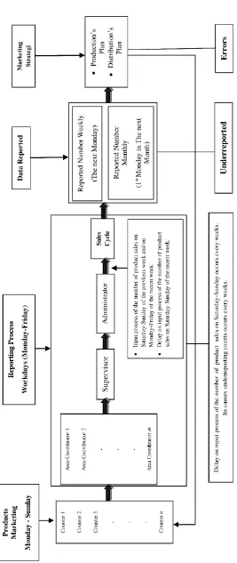
In this research, underreported counts occurred as a result of delay on input process of the number of product sales repeatedly. In this system (see Figure 1), the input process of the number of product sales will directly reduce the stock number of the products in the counter. That would indirectly lead to over reporting the stock number the products in the counter. This is a major factor that caused errors on the next production's plan or in the distribution of products. In order to reduce the risks, the actual number of product sales is need to be estimated.

The consequence of the underreporting counts is the number of product sales reported is only part of the actual number of product sales. There are a number of product sales which are unreported. It means that a product sold at a counter will have two possible treatments from the administrator i.e. inputted into the system or not. An opportunity for a product sold at a counter inputted to the system called probability of reported. This probability has a value ranging from 0-1. It is also known that the actual number of product sales in a counter within a month was random and ranged between 0-21 pieces with an average of 4 pieces per month. Both of the information can be considered as a prior information that can be used in the estimation of the actual number of product sales.

The actual number of product sales is influenced by the activity of selling the product itself. As cited in Sinaga (2013), one of the factors that affects sales activities is market conditions (Basu, 2005). The market conditions can be seen as a rate of product sales at its counter. Thus, to estimate the actual number of product sales, need an analysis that can describe the relationship between the number of products sales (underreported) with rate of product sales involving both the prior information before.

So far modeling of the count data using Poisson regression model and binomial regression models. However, both models can be used if the count data is considered accurately reported. As cited in Papadatos (2005), models for under-reported counts were first introduced in Moran's characterization (1952) and Rao-Rubin condition (1964). Then, several researchers have developed a model for underreported counts, including the Poisson regression model for underreported counts developed by Winkelmann (1996), Mukhopadhyay (1997) developed the negative binomial regression model for underreported counts (as cited in Pararai, 2010) and the generalized Poisson-Poisson mixture models which can be used for misreporting counts (under, over and accurately reported) developed by Pararai (2010).

2. Poisson Model for Underreported Counts

Moran (1952) introduced a characterization of underreported counts (as cited in Papadatos, 2005). It is stated that if N1 and N2 are non-degenerate independent

random variables and its values are non-negative and if the conditional distribution of

N1 (N1+N2 =n) is binomial and its parameter is n N



0,1,



with success probability

0,1

p



_ _ for some

n N



,

P N

_{ 1}



N

₂



n

_



0

then the distributions of

N N

₁

,

₂ and



N

1



N

2



n



are Poisson. For some

i



N

,

P N

 1

 

i



0

and

P N

 2

 

i



0

.

Another form of Moran's (1952) characterization was introduced by Rao and Rubin (1964), independence of N1and N2 called as Rao-Rubin condition. For some

p





0,1



, then Rao-Rubin condition implies that N1 and N2 follow a Poisson distribution with

parameter



p

and





1



p



for some





0

.

3. Poisson Regression Model for Underreported Counts

Poisson regression model for underreported counts which is developed by Winkelmann (1996) was also a mixture of binomial distribution and Poisson distribution.

Let

Y

_i* as an actual number of observed events in a specific time for individual i.

Assume that

Y

_i* depends on

x

_i and follows a Poisson distribution with parameter

exp

.

i i





_

x



β

_{ Let}

i

Y

as the reported number of observed events in a specific time for individual i and follows a binomial distribution with parameters

Y

_i* and p (probability of reported).

Underreported countsoccur if

Y

_i*



Y

_i so the marginal distribution of

Y

i is a Poisson

regression model with parameter



_i

p



exp

_

x

_i



β

_



p

.

Parameter pi cannot be treated as a fixed parameter since the model is singular

with n+k parameter and n data points (Winkelmann, 1996). To solve this problem, Winkelmann consider the parameter pi as a random variabel which follows a certain

distribution. Further, Winkelmann (1996) obtained the posterior distribution of y*_{, p and} β as:



*





*



 

*

   

, ,

,

,

posterior _likelihood prior

P y p

β x

y



P y y p



P y

β



f

β



f p

(1)

Drapper & Guttman (1971) assume that the parameters N and p are independent random variables, where N follows a discrete uniform distribution and p follows a beta distribution (as cited in Moreno, 1998). Meanwhile, Raftery (1988) assumes that N

follows a Poisson distribution with parameter λ and p follows a uniform distribution (as cited in Moreno, 1998). Winkelmann (1996) assumes that N or _Y* _{follows a Poisson}





 

 

 









 

 

 

*_{, ,} *_, * 1 ₁ exp 2 * 1 *

exp exp .

* _{! !} 1

P Y_i p Y_{i i} P Y Y_{i i} p_i P Y_i f f p_i

y_i y_i y_i

p p

n _{i i}

y_{i i i}

y y y

i _{i i i}

        _    _    _      _{ }     _   _{ }   _  β β β β μ β μ

xβ x β

(2)

with *

0,1, 2, ; 0,1, 2, ; 0 1; ; 1, 2, ,

i i i

Y  Y   p      β i n

4. Markov Chain Monte Carlo (MCMC)

MCMC is done by drafting markov chain that converges quickly on the posterior distribution. MCMC generate sample data of parameter θ which has a spesific distribution through an algorithm and done iteratively (the value of each step depends on the previous step). Gibbs sampling is one of the MCMC algortihm which usually used. Gibss sampling can be applied if the conditional distribution of each parameter is known.

Estimation of the paramater of the model using MCMC will depend on the determination of the burn in period, which is done in line with determination the convergence of the algorithm using trace plot, autocorrelation plot and ergodic mean plot.

Base from the posterior distribution developed by Winkelmann, it is obvious that it is difficult to determine the kind of posterior distribution. To facilitate the parameter estimation, Markov Chain Monte Carlo (MCMC) simulation with full conditional distribution is used as given in the Winkelmann (1996). The MCMC Algorithm is as follows :

1. Set the initial value of each parameters

Y

* 0 

,

p

 0 and

β

 0

2. Set the number of iteration T

3. For t = 1, 2, …, T repeat the following steps :

a. Generate new candidate of

Y

_i* t from *

   

t 1

,

t 1

,

i i i

Y

β



p



Y

b. Generate new candidate of

p

_i t from

,

* t

i i i

p Y Y

c. Generate new candidate of

β

 t from

β

Y

_i* t

,

Y

_i using Random-Walks

algorithm with  t  t 1 12            

β β V z and

z

~

N

_D

 

0 I

,

4. Update the values of each parameter using the values obtained by the simulation.

5. Check the convergence of the algorithm using Autocorrelation plot, Trace plot and Ergodic mean plot

6. Determine the burn in period.

a. The average value and standard deviation of the parameter

β

b. The average value and standard deviation of the parameter

p

_i for

1, 2,

,

i



n

c. The average value and standard deviation of the parameter

Y

_i*for

1, 2,

,

i



n

5. Results and Discussion

The data used in this study is product sales at 108 counters in August 2013 of a garment company in Bandung City, Indonesia. These counters belong to the group of regions that have the highest sales target compared with other counters across of Indonesia. The rate of product sales of these counters was also the highest compared with others. This causes the risk of delay on input process is very high, while the products distributions must run every week and production plans run every month (see Figure 1). This is a major factor that lead in increasing the errors on the marketing strategies (se Figure 1). In order to reduce the risks, the actual number of product sales is need to be estimated.

Count variable, reported number of product sales has values between 1-26 pieces with an average of 5.44 and standard deviation 4.57. While the independent variable is the rate of products sales in each counter and divided into 4 categories such as very high, high, low and very low. Therefore, the regression model of the actual number of product sales involved 3 dummy variables. MCMC simulation performed with 5000 iterations and the algorithm before. To check the convergence of the series we use trace plot, autocorrelation plot and ergodic mean plot.

All the trace plot (simulation p, simulation Y* _{and simulation} β_{) did not show a certain}

pattern. The autocorrelation plots (simulation p, simulation Y* _{and simulation} β_{) showed}

there are not an autocorrelation between two iterations. Ergodic mean plots showed that ergodic mean of the sample values of parameter p, Y* _and β _{are stabilize after the}

first 3000 iterations. Then, the convergence of the simulation for parameter p and Y*

and regression parameter β has been achieved with the burn in period of 3000 first iterations.

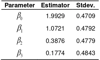
From the simulations, the results of the regression parameter estimation can be seen in Table 1 below:

Table 1: Regression Parameters Estimate

Parameter Estimator Stdev.

0



1.9929 0.4709

1



1.0721 0.4792

2



0.3876 0.4779

3



0.1774 0.4843

1,9929+1,0721 ₁ +0,3876 ₂ +0,1774 ₃ *

ˆ Di D i D i _.

E Y X e

i i i

 _ _  

 

 

Therefore, based on the category rate of products sales in each counters, the estimates of the average of the actual number of the product sales in August 2013 can be seen in Table 2.

The mean values of product sales, obtained from the above regression equation, presented in the above table. It can be seen that the average of the actual number of the product sales in August 2013 at the counter with the rate of product sales very high is 21 pieces, at the counter with the rate of product sales high is 11 pieces, at the counter with the rate of product sales low is 9 pieces and at the counter with the rate of product sales very low is 7 pieces.

Tabel 2: The Estimators of The Mean of The Actual Number of The Product Sales

The Rate Of Product Sales

*

ˆ

i E Y Xi i

 _{ } _

Very High 21

High 11

Low 9

Very Low 7

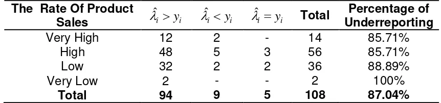
To determine the possibility occurences of underreporting counts, we compared the estimated value of the average of the actual number of the product sales (see Table 2) with the number of product sales recorded in the report (underreported counts). The results (see Table 3) show that the product sales of 87.04% counters from 108 are run into underreporting counts. It means that the risk of error in the production's plans, product distributions or in other marketing strategies will be high.

Tabel 3: The Comparison of The Estimators of The Average of The Actual Number of The Product Sales on Product Sales Report (Underreported Counts)

The Rate Of Product

Sales



ˆi yi



ˆi yi



ˆi yi Total

Percentage of Underreporting

Very High 12 2 - 14 85.71%

High 48 5 3 56 85.71%

Low 32 2 2 36 88.89%

Very Low 2 - - 2 100%

Total 94 9 5 108 87.04%

Meanwhile, the results of the estimation of the actual number of the product sales or *

Y and the probability for a product sold reported (inputted to the system) or p based on the category the rate of products sales in each counter are in the following Table 4, Table 5, Table 6 and Table 7.

Tabel 4 : The Estimators of Model Parameter at Counter with The Very High Rate of Product Sales

Counter 𝑦_𝒊 𝑦̂_𝑖∗ 𝑠𝑡𝑑(𝑦̂)_𝑖 ̂𝑝_𝑖∗ 𝑠𝑡𝑑(𝑝̂)_𝑖∗ 𝑞̂𝑥100%_𝑖∗

𝑦̂ ±𝑖∗

𝑠𝑡𝑑(𝑦̂)𝑖

[𝑦̂ ±𝑖∗

𝑠𝑡𝑑(𝑦̂)] − 𝑦𝑖 𝒊

Counter 1 15 21 4 0.7122 0.1533 28.78% 17-26 2-11 Counter 2 1 21 5 0.0957 0.0696 90.43% 15-26 14-25 Counter 3 23 26 3 0.8648 0.1052 13.52% 23-29 0-6 Counter 4 11 21 5 0.5583 0.1638 44.17% 16-26 5-15 Counter 5 4 21 5 0.2299 0.1037 77.01% 16-26 12-22 Counter 6 1 21 5 0.0925 0.0655 90.75% 15-26 14-25 Counter 7 8 21 5 0.4234 0.1435 57.66% 15-26 7-18 Counter 8 5 21 5 0.2804 0.1196 71.96% 16-26 11-21 Counter 9 13 21 5 0.6445 0.1633 35.55% 16-26 3-13 Counter 10 4 20 5 0.2362 0.1087 76.38% 15-26 11-22 Counter 11 26 28 3 0.8929 0.0857 10.71% 26-31 0-5 Counter 12 1 20 5 0.0959 0.0681 90.41% 15-26 14-25 Counter 13 3 21 5 0.1852 0.096 81.48% 15-26 12-23 Counter 14 5 21 5 0.2839 0.1181 71.61% 15-26 10-21

Average 9 22 5 0.3997 0.1117 60.03% 17-26 8-18

From Table 5, we get that the average of the estimators of the actual number of the product sales at a counter with the rate of product sales high is ranging between 8-14 pieces with a gap of 3-8 pieces compared to the number of the product sales listed in the report (obtained from the system). The mean percentage of underreporting counts of product sales is 50.29% or ranged from 9.09% to 81.87%.

Tabel 5 : The Estimators of Model Parameter at Counter with The High Rate of Product Sales

Counter 𝑦_𝒊 𝑦̂_𝑖∗ 𝑠𝑡𝑑(𝑦̂)_𝑖 ̂𝑝_𝑖∗ 𝑠𝑡𝑑(𝑝̂)_𝑖∗ 𝑞̂𝑥100%_𝑖∗ 𝑦̂ ±_𝑖∗ 𝑠𝑡𝑑(𝑦̂)𝑖

[𝑦̂ ±𝑖∗

𝑠𝑡𝑑(𝑦̂)] − 𝑦𝑖 𝒊

Counter 𝑦_𝒊 𝑦̂_𝑖∗ 𝑠𝑡𝑑(𝑦̂)_𝑖 ̂𝑝_𝑖∗ 𝑠𝑡𝑑(𝑝̂)_𝑖∗ 𝑞̂𝑥100%_𝑖∗ 𝑦̂ ±_𝑖∗ 𝑠𝑡𝑑(𝑦̂)𝑖

[𝑦̂ ±𝑖∗

𝑠𝑡𝑑(𝑦̂)] − 𝑦𝑖 𝒊

Counter 17 13 15 2 0.8484 0.1157 15.16% 13-16 0-3 Counter 18 3 10 3 0.3776 0.1865 62.24% 6-13 3-10 Counter 19 3 10 3 0.3544 0.1683 64.56% 7-13 4-10 Counter 20 7 11 3 0.6443 0.1831 35.57% 8-14 1-7 Counter 21 10 12 2 0.7844 0.1449 21.56% 10-15 0-5 Counter 22 14 16 2 0.8652 0.1069 13.48% 14-17 0-3 Counter 23 7 11 3 0.6487 0.1872 35.13% 8-14 1-7 Counter 24 3 10 3 0.3707 0.1777 62.93% 6-13 3-10 Counter 25 6 10 3 0.599 0.1941 40.10% 7-13 1-7 Counter 26 5 10 3 0.5168 0.1856 48.32% 7-14 2-9 Counter 27 11 13 2 0.8085 0.1387 19.15% 11-15 0-4 Counter 28 3 10 3 0.3723 0.1823 62.77% 6-13 3-10 Counter 29 1 10 3 0.1833 0.1307 81.67% 7-13 6-12 Counter 30 2 10 3 0.2747 0.1628 72.53% 7-13 5-11 Counter 31 6 11 3 0.5893 0.186 41.07% 8-14 2-8 Counter 32 10 13 2 0.7666 0.1514 23.34% 10-15 0-5 Counter 33 12 14 2 0.8394 0.1216 16.06% 12-16 0-4 Counter 34 2 10 3 0.2812 0.1589 71.88% 6-13 4-11 Counter 35 8 11 3 0.6985 0.1715 30.15% 9-14 1-6 Counter 36 1 10 3 0.1822 0.1252 81.78% 7-13 6-12 Counter 37 6 10 3 0.5994 0.189 40.06% 7-13 1-7 Counter 38 4 10 3 0.4421 0.1903 55.79% 7-13 3-9 Counter 39 1 10 3 0.185 0.1326 81.50% 7-13 6-12 Counter 40 2 10 3 0.2744 0.1582 72.56% 6-13 4-11 Counter 41 2 10 3 0.273 0.1582 72.70% 6-13 4-11 Counter 42 7 11 3 0.661 0.1858 33.90% 8-13 1-6 Counter 43 2 10 3 0.2775 0.1608 72.25% 7-13 5-11 Counter 44 7 11 3 0.6493 0.1855 35.07% 8-14 1-7 Counter 45 2 10 3 0.2743 0.1612 72.57% 7-13 5-11 Counter 46 2 10 3 0.2821 0.1589 71.79% 6-13 4-11 Counter 47 8 11 3 0.7136 0.1718 28.64% 9-14 1-6 Counter 48 1 10 3 0.1833 0.1291 81.67% 7-13 6-12 Counter 49 4 10 3 0.444 0.1847 55.60% 7-13 3-9 Counter 50 4 10 3 0.4573 0.1949 54.27% 7-13 3-9 Counter 51 2 10 3 0.2671 0.1521 73.29% 7-13 5-11 Counter 52 3 10 3 0.3687 0.1827 63.13% 7-13 4-10 Counter 53 7 11 3 0.6523 0.1822 34.77% 8-14 1-7 Counter 54 3 10 3 0.3651 0.1774 63.49% 7-13 4-10 Counter 55 5 10 3 0.5348 0.19 46.52% 7-13 2-8 Counter 56 4 10 3 0.4511 0.1943 54.89% 7-13 3-9

Average 5 11 3 0.4971 0.1639 50.29% 8-14 3-8

the report (obtained from the system). The mean percentage of underreporting counts of product sales is 49.20% or ranged from 11.70% to 77.46%.

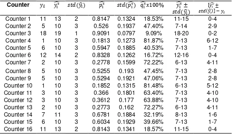
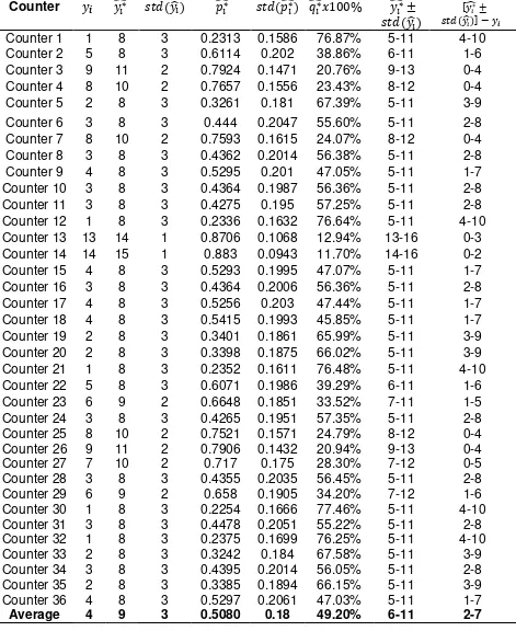
Tabel 6: The Estimators of Model Parameter at Counter with The Low Rate of Product Sales

Counter 𝑦_𝒊 𝑦̂_𝑖∗ 𝑠𝑡𝑑(𝑦̂)_𝑖 ̂𝑝_𝑖∗ 𝑠𝑡𝑑(𝑝̂)_𝑖∗ 𝑞̂𝑥100%_𝑖∗ 𝑦̂ ±_𝑖∗ 𝑠𝑡𝑑(𝑦̂)𝑖

[𝑦̂ ±𝑖∗

𝑠𝑡𝑑(𝑦̂)] − 𝑦𝑖 𝒊

Counter 1 1 8 3 0.2313 0.1586 76.87% 5-11 4-10 Counter 2 5 8 3 0.6114 0.202 38.86% 6-11 1-6 Counter 3 9 11 2 0.7924 0.1471 20.76% 9-13 0-4 Counter 4 8 10 2 0.7657 0.1556 23.43% 8-12 0-4 Counter 5 2 8 3 0.3261 0.181 67.39% 5-11 3-9 Counter 6 3 8 3 0.444 0.2047 55.60% 5-11 2-8 Counter 7 8 10 2 0.7593 0.1615 24.07% 8-12 0-4 Counter 8 3 8 3 0.4362 0.2014 56.38% 5-11 2-8 Counter 9 4 8 3 0.5295 0.201 47.05% 5-11 1-7 Counter 10 3 8 3 0.4364 0.1987 56.36% 5-11 2-8 Counter 11 3 8 3 0.4275 0.195 57.25% 5-11 2-8 Counter 12 1 8 3 0.2336 0.1632 76.64% 5-11 4-10 Counter 13 13 14 1 0.8706 0.1068 12.94% 13-16 0-3 Counter 14 14 15 1 0.883 0.0943 11.70% 14-16 0-2 Counter 15 4 8 3 0.5293 0.1995 47.07% 5-11 1-7 Counter 16 3 8 3 0.4364 0.2006 56.36% 5-11 2-8 Counter 17 4 8 3 0.5256 0.203 47.44% 5-11 1-7 Counter 18 4 8 3 0.5415 0.1993 45.85% 5-11 1-7 Counter 19 2 8 3 0.3401 0.1861 65.99% 5-11 3-9 Counter 20 2 8 3 0.3398 0.1875 66.02% 5-11 3-9 Counter 21 1 8 3 0.2352 0.1611 76.48% 5-11 4-10 Counter 22 5 8 3 0.6071 0.1986 39.29% 6-11 1-6 Counter 23 6 9 2 0.6648 0.1851 33.52% 7-11 1-5 Counter 24 3 8 3 0.4265 0.1951 57.35% 5-11 2-8 Counter 25 8 10 2 0.7521 0.1571 24.79% 8-12 0-4 Counter 26 9 11 2 0.7906 0.1432 20.94% 9-13 0-4 Counter 27 7 10 2 0.717 0.175 28.30% 7-12 0-5 Counter 28 3 8 3 0.4355 0.2035 56.45% 5-11 2-8 Counter 29 6 9 2 0.658 0.1905 34.20% 7-12 1-6 Counter 30 1 8 3 0.2254 0.1666 77.46% 5-11 4-10 Counter 31 3 8 3 0.4478 0.2051 55.22% 5-11 2-8 Counter 32 1 8 3 0.2375 0.1699 76.25% 5-11 4-10 Counter 33 2 8 3 0.3242 0.184 67.58% 5-11 3-9 Counter 34 3 8 3 0.4395 0.2014 56.05% 5-11 2-8 Counter 35 2 8 3 0.3385 0.1894 66.15% 5-11 3-9 Counter 36 4 8 3 0.5297 0.2061 47.03% 5-11 1-7

Average 4 9 3 0.5080 0.18 49.20% 6-11 2-7

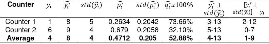
4-13 pieces with a gap of 1-9 pieces compared to the number of the product sales listed in the report (obtained from the system). The mean percentage of underreporting counts of product sales is 52.88% or ranged from 32.10% to 73.66%.

Tabel 7: The Estimators of Model Parameter at Counter with The Very Low Rate of Product Sales

Counter 𝑦_𝒊 𝑦̂_𝑖∗ 𝑠𝑡𝑑(𝑦̂)_𝑖 ̂𝑝_𝑖∗ 𝑠𝑡𝑑(𝑝̂)_𝑖∗ ̂𝑥100%𝑞∗_𝑖 𝑦̂ ±_𝑖∗ 𝑠𝑡𝑑(𝑦̂)𝑖

[𝑦̂ ±𝑖∗

𝑠𝑡𝑑(𝑦̂)] − 𝑦𝑖 𝒊

Counter 1 1 8 5 0.2634 0.2042 73.66% 3-13 2-12 Counter 2 6 9 4 0.679 0.2058 32.10% 5-13 0-7

Average 4 8 4 0.4712 0.205 52.88% 4-13 1-9

6. Conclusion

The estimation of the parameters of the regression model for underreported counts performed through by a Bayesian approach and Markov Chain Monte Carlo simulation using Gibbs sampling algorithm, is depend on the determination of burn in period. Determination of burn in period or deleting the first B iterations of the algorithm is done to reduce or avoid the effect of the initial value of the specified parameter. These initial values may affect the posterior summary if they have a huge gap from the highest value of the posterior probability.

Determination of burn in period is done in line with the convergence of algorithm conducted through trace plot, autocorrelation plot and ergodic mean plot. The determination of burn in period is easier using ergodic mean plot than using the trace plot or autocorrelation plot. Ergodic mean plot describes the average simulation values on current iteration. Then, the researcher can more easily determine the first B

iterations to be removed. While the trace plot only illustrates the randomness pattern of simulated results and autocorrelation plot only describes the value of autocorrelation between successive iterations. After burn in period is determined, the estimated value of the underreported model parameters is the average of the simulated sample values of each parameter calculated from sample value after burn in period until the last iteration.

The results of estimation clearly showed the percentage of underreporting counts is very high, either on the counter whose sales rate is very high, high, low or very low. it also showed a gap between undamaged product sales and the actual number. The gap is the number of damaged product sales. In order to reduce the risks of the errors on the marketing strategies (see Figure 1), these estimation value can be more useful.

References

Moreno, E., and Giron, J. (1998). Estimating with incomplete count data A Bayesian approach. Journal of Statistical Planning and Inference, 66(1), 147-159.

Neubauer, G., Djuraš, G., and Friedl, H. (2011). Models for underreporting: A Bernoulli

sampling approach for reported counts. Austrian journal of statistics, 40(1&2), 85-92.

Papadatos, N. (2005). Characterizations of discrete distributions using the Rao–Rubin

Pararai, M., Famoye, F., and Lee, C. (2010). Generalized poisson-poisson mixture

model for misreported counts with an application to smoking data. Journal of Data

Science, 8(4), 607-617.

Sinaga, U. I. (2013). Faktor–Faktor yang Mempengaruhi Volume Penjualan Sepeda

Motor Honda Vario pada PT. Capella Dinamik Nusantara Pekanbaru. Riau

University, Pekanbaru.

Winkelmann, R. (1996). Markov chain Monte Carlo analysis of underreported count

data with an application to worker absenteeism. Empirical Economics, 21(4),