ANALYSIS OF ROAD DAMAGE DUE TO OVER LOADING
(CASE STUDY: DEMAK -TRENGGULI ARTERIAL ROAD,
CENTRAL JAVA PROVINCE, INDONESIA)
Thesis
Submitted as Partial Fulfilling of the Requirement for the Degree of Master of Civil Engineering Diponegoro University
IBRAHIM ABOBAKER ALI LANGER NIM: L4A909002
STATEMENT OF AUTHENTIFICATION
Herewith I stated that this thesis has never been published in other institution and there were no part of this thesis has been directly copied from published sources except citing from listed bibliographies attached.
Semarang, February 2011
DEDICATION
To all those who love me and those that I love.
ACKNOWLEDGEMENTS
First and foremost, I would like to thank Allah S.W.T for giving me strength to endure the challenges i]n my quest to complete this research.
Secondly, I would like to thanks my supervisors, Ir. Bambang Pudjianto, MT. and Dr. Bagus Hario Setiadji, ST., MT. for their advice, patience and guidance throughout the process of completing this research. And thankful the head of master program Dr. Bambang Riyanto, DEA. for his kind help and support, and to all my lecturers who had taught me in DIPONEGORO UNIVERSITY, thank you for all the knowledge and guidance.
Also I would like to thank to my beloved family members. Their support was instrumental for the successful completion of this research project.
ABSTRACT
The ability of a pavement structure in carrying out its function reduces in line with the increase of traffic load, especially if there are overloaded heavy vehicle passing through the road. In this thesis, the effect of overloaded vehicles on the road pavement service life was analyzed using the AASHTO 1993. Vehicle damage factor (VDF) and Structural Number (SN) were calculated on normal and overloading conditions. Remaining of pavement service life due to overloading condition was also presented. So it can be concluded how severe the effect of overloaded vehicles against pavement service life.
In this thesis it can be seen, that the presence of overloaded vehicles, particularly heavy vehicles (class 6B up to class 7C according to Bina Marga’s vehicle classification) resulted in traffic load (W18) value that was 200% greater than that of standard load condition. The increase of W18 value can affect the pavement service life. For the direction of Demak Trengguli, the pavement service life reduced by 70% due to overloading condition, while for the opposite direction, the service life was reduced by 40% caused by the same factor. In terms of layer thickness, overloading condition also increase the layer thickness than that of thickness at the load legal limit 10 ton. For the direction of Demak-Trengguli, the thickness reached 186% higher than of standard design, while for the direction of Trengguli-Demak, it’s obtained that due to overloading condition, the layer thickness approximately 177% higher than that of standard design.
From the results, it can be concluded that overloaded vehicles on the road are very influential to the reduction in pavement service life. Therefore, it is expected that road users to comply with existing regulations in the conduct of transportation.
Key words: overload vehicle, damage factor, pavement service life, pavement thickness.
2.3.5 Sub grade Bearing Capacity MR ... 14
2.3.6 Structural Number ... 15
2.3.7 Determination of Structural Number ... 20
2.4 Equivalent Single Axle Load Factor ... 20
2.5 Previous of Studies ... 22
4.2. Determination of Vehicle Damage Factor (VDF) ... 28
4.3 Calculation of Traffic Load ... 32
4.4 Reduction of Pavement Service Life ... 33
4.5 Calculation of Structural Capacity ... 37
4.5.1 Loss of Serviceability (∆PSI) ... 37
4.5.2 Resilient modulus (MR) ... 38
4.5.3 Calculation of Structural Number (SN) and Layer Thickness (D) ... 39
CHAPTER 5 CONCLUSIONS AND RECOMMENDATIONS ... 43
5.1 Conclusions ... 43
LIST OF TABLES
Table 0.1 Lane Distribution Factor (DD) ... 10
Table 0.2 Recommendation of Reliability Level for Various Road Classifications ... 13
Table 2.3 Standard Normal Deviation for certain reliability service ... 14
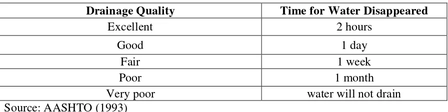
Table 2.4 The Definition of Drainage Quality... 16
Table 2.5 Drainage Coefficient (m) ... 16
Table 4.1 ADT for heavy vehicles ... 27
Table 4.2 Axle load Equivalency Factor For Flexible Pavement Single Axle and Pt of 2.0.. ... 29
Table 4.3 Axle load Equivalency Factor For Flexible Pavement tandem Axle and Pt of 2.0. ... 30
Table 4.4 Axle load Equivalency Factor For Flexible Pavement triple Axle and Pt of 2.0 ... …31
Table 4.5 Total VDF for all Heavy Vehicle Classes ... 32
Table 4.6 Traffic load (as designed and overloaded condition) ... 33
Table 4.7 Relationship between Traffic Load and Service Life ... 36
Table 4.8 Loss of Serviceability for Demak – Trengguli Direction ... 37
Table 4.9 Loss of Serviceability for Trengguli – Demak Direction ... 37
Table 4.10 Modulus Resilient of Subgrade ... 39
Table 4.11 SN and Layer Thickness of Road of Demak - Trengguli Direction (Standard Condition) ... 40
Table 4.12 SN and Layer Thickness of Road of Demak - Trengguli Direction (Overloaded Condition) ... 41
LIST OF FIGURES
Figure 1.1 Location Map of Northern Regions (Demak-Trengguli) ... 3
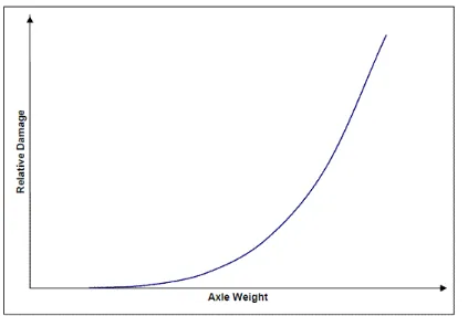
Figure 2.1 The fourth Power Relationship between Axle Weight and Pavement Damage ... 7
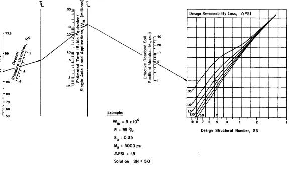
Figure 2.2 AASTHO Fexble Pavement Design Nomograph .(AASHTO 1993) ... 8
Figure 2.3 Relative Strength Coefficient of Asphalt Concrete Surface Course ... 18
Figure 2.4 Variation of Relative Strength Coefficient of Granular Base Layers (a2) ... 18
Figure 2.5 Variation of Relative Strength Coefficient of Granular Subbase Layers (a3) ... 19
Figure 06 Variation of Relative Strength Coefficient of Cement-Treated Base (a2) ... 19
Figure 0 Variation of Relative Strength Coefficient of Asphalt-Treated Base (a2) ... 20
Figure 3.1 Methodology of This Study ... 25
Figure 4.1 Service Relationship between Traffic Load and Service Life on Standard and Overloaded Conditions (Demak – Trengguli Direction) ... 34
NOMENCLATURE
a Layer coefficient
ADT Average daily traffic
PSI Loss of serviceability
Swell rate constant
CHAPTER 1 INTRODUCTION
1.1 Background
Pavements are engineering structures placed on natural soils and designed to withstand the traffic loading and the action of the climate with minimal deterioration and in the most economical way (Hudson et al., 2003). The majority of modern pavement structures may be classified as flexible or rigid pavement structures. A flexible pavementconsists of a surface layer constructed of flexible materials (typically asphalt concrete) over granular base and sub base layers placed on the existing, natural soil. Rigid pavement is a pavement structure that deflects very little under loading because of the high stiffness of the Portland cement concrete used in the construction of surface layer. The rigid pavements can be further categorized depending on the types of joints constructed and use of steel reinforcement (Gillespie, 1993).
Each of these pavement types has specific failure mechanisms and each failure mechanism is caused by specific factors. Example of such failure mechanisms include: fatigue damage and roughness of rigid and flexible pavements, faulting of rigid pavements, and rutting of flexible pavements. These failure mechanisms are caused by the following factors: heavy vehicle loadings, climate, drainage, materials properties, and inadequate layer thicknesses (Hudson et al., 2003).
Among these factors, heavy vehicle loads are the major source for pavement damage. Magnitude and configuration of vehicular loads together with the environment have a significant effect on induced tensile stresses within flexible pavement (Yu et al., 1998).
to the road pavement. Regulators need to allocate costs to vehicle operators in accordance with truck-induced damage to pavements. The proper evaluation of truck damage also helps the highway engineers in the optimization of pavement design and maintenance activities (Zaghloul and White, 1994).
In recent years, several studies have estimated the truck damage by computing the responses (stresses, strains and deflections) of pavements under heavy vehicles loadings using mechanistic approaches (Chen et al., 2002). In response to the need for mechanistic pavement design and analysis procedures, researchers are increasingly using three dimensional finite element analysis techniques to quantify the response of the pavement system to applied axle and temperature loading (Davids, 2000).
Another tool that would allow estimating the truck damages is the new Mechanistic Empirical Design Guide for pavements. Due to its advanced modeling capabilities, it is expected that federal and state transportation agencies will phase out the old empirical AASHTO Pavement Design Guide (1986, 1993) to let the new Mechanistic Empirical Design Guide handle nowadays pavement design challenges such as increased number and weight of heavy vehicles (FHWA, 2005).
The length of the bulge front/rear, Height of vehicles, will impact on increasing the carrying capacity of vehicles. Furthermore, this will directly increase load axis of the vehicle, so that the axle load will be heavier than the permitted (legal limit). This raises the problem of excessive load or overloading. The impact of overload conditions on the road pavement is premature failure, that is, a condition which the damage can reduce the life of roads before the design life of the road is reached. Research on excess load showed that it could significantly accelerate the damaging effect to the roads and endangering the safety of road users (Badan Litbang Departement PU, 2004)
1.2 The Location of Research
Figure1.1: Location of Demak-Trengguli Road Segment
1.3 Research Questions
b. What is the difference in pavement service life between two conditions: road under standard traffic load and overloading condition?
1.4 Objectives
The objective of this research is to analyze the effect of overloaded heavy vehicle to the road pavement damage. The objective can be detailed into two targets:
a. To determine the reduction of pavement service life on the Demak-Trengguli road segment due to overloading.
b. To calculate the layer thicknesses required by pavement structure to withstand against overloading condition.
1.5 Research Scope and Limitations
In this study, the research scope and limitations are as follows.
a. The case study investigated in this research is Demak - Trengguli road segment, that is a two-way four-lane divided (4/2 D) flexible pavement road.
b. The calculation of pavement service life is based on ADT and CESAL of overloaded truck;
c. The standard method used in this study is AASHTO 1993
1.6 Organization of Thesis
In accordance with the Master Program, the proposal is organized into five chapters as follows:
Chapter 1 Introduction
This chapter consists of background, purpose, objectives, and location of case study.
Chapter 2 Literature Review
This chapter describes about characteristic of traffic, transport mode, the factors causing road damage and vehicle damage factor as well as pavement thickness design.
Chapter 3 Methodology
This chapter presents the descriptions of the approaches being taken to achieve objectives included in the secondary data processing, data analysis, and evaluation of results.
This chapter contains the data analysis due to overload, so that it will know how severe the overloaded truck will affect the road segment that is concerned.
Chapter 5Conclusion and Recommendation
CHAPTER 2 LITERATURE REVIEW
2.1 Background
The current flexible pavement design methodology used by Bina Marga (Directorate General of Highway, DGH) is derived from the results of the American Association of State
Highway Officials (AASHO) Road Test, conducted in the late 1950’s. A basic nomograph
ESAL values for other axles express their relative effect on pavement structure. If the number and types of vehicles using the pavement can be predicted, then engineers can design the pavement for anticipated a number of 18 kips equivalent single axle loads (18 kips ESAL). Virtually, all heavy-duty pavements built in the United States since the mid-1960s have been designed using the principles and formulas developed from the Road Test (Davis, 2009).
The test vehicles ranging in gross weight from 2,000 lb to 48,000 lb. The improved paving materials that are used today such as Superpave mixes, stone mastic asphalts, and open graded friction courses were not available during the road test. Within the pavement cross section, only one type of HMA, granular base material, and sub grade soil were used. The thickest HMA pavement was 6 inches. All results from the road test are a product of the climate of northern Illinois within a two-year period (HRB, 1962).
2.2.2 Results of AASHO Road Test
The results of the AASHO Road Test were used to develop the first pavement design guide, known as the AASHO Interim Guide for the Design of Rigid and Flexible Pavements. This design guide was issued in 1961, and had major updates in 1972, 1986, and 1993. The 1993 AASHTO Design Guide is essentially the same as the 1986 Design Guide for the design of new flexible pavements, and is still used today by many transportation agencies, including Bina Marga.
Figure 2.1: The Fourth Power Relationship between Axle Weight and Pavement Damage (HRB,1962)
2.3 Fundamental Equations
The 1993 AASHTO Design Guide is the current standard used for designing flexible pavement for many transportation agencies. In the AASHTO design methodology, the subgrade resilient modulus (MR), applied ESAL (W18), reliability (with its associated normal
(2.1)
2.3.1 Traffic Load, W18 and Growth Rate, Gr
Wt is the number of single-axle load applications to cause the reduction of serviceability to the terminal level (pt). and The standard deviation, So, is typically assumed to be 0.49 for flexible pavements based upon previous research (AASHTO, 1993).
Traffic load that used for determining flexible pavement design thickness in 1993 AASHTO is the cumulative traffic load during design life. The magnitude of the traffic load for two ways is obtained by summing the multiplication of three parameters, i.e. average daily traffic, axle load equivalency factor, and annual growth rate, for each type of axle load. Numerically, the formulation of cumulative traffic load is as follows:
x x GRi
x 365W = cumulative standard single axle loads for two ways, ESALs ADTi = average daily traffic for axle load i
Ei = axle load equivalency factor (or vehicle damage factor) for axle load i GRi = annual growth rate for vehicle i, %
gi = traffic growth for vehicle type i (%) n = service life, year
To obtain traffic on the design lane, the following formulation can be used:
where:
W18 = cumulative standard single axle load on design lane, ESAL DD = direction distribution factor
DL = lane distribution factors
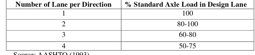
DD is generally taken 0.5. In some special cases, there are exceptions where heavy vehicles tend to run on a certain direction. Several studies indicate that the DD varies from 0.3 to 0.7 depending on which direction that considers as major and minor (AASHTO 1993). The magnitude of DL is determined based on the number of lanes in one carriageway (see Table 2.1)
Table 2.1: Lane Distribution factor (DL)
Number of Lane per Direction % Standard Axle Load in Design Lane
1 100 required to extend its service life. The equation of PSI is given by:
PSI = PSItraffic + PSISW, FH (2.4)
IPt = 2,5 - 3,0 for major highway and pt equals to 2 for minor highway
PSISW, FH = serviceability loss because of soil swelling (effect of moisture and frost)
ΔPSISW, FH = 0,00335 . VR . PS . (1 – e-t) (2.5)
= swell rate constant (as a function of moisture supply and soil fabric)
VR = maximum potential heave (as a function of plasticity index, compaction and
subgrade thickness), inch.
Ps = swelling probability, %
2.3.3The Relationship between PSI and IRI
The loss of serviceability (ΔPSI) is the difference between the initial serviceability of the pavement when opened to traffic and the terminal serviceability that the pavement will reach before rehabilitation, resurfacing or reconstruction is required. The present serviceability index (PSI), also known as the present serviceability rating (PSR), is a subjective measure by the road user of the ride quality, ranging from zero (impassible) to five (perfect ride). Studies conducted at the AASHO Road Test found that for a newly constructed flexible pavement, the initial serviceability (po) was approximately 4.2 (AASHTO, 1993).
The value of a terminal serviceability (pt) was ranging between 2.0 and 3.5. The 1993 AASHTO Design Guide recommends the selection of pt based upon the same traffic levels used for reliability selection: for low traffic, 2.5, for medium traffic, 3.0, and for high traffic, 3.5. To demonstrate the subjectivity of the measurement, studies from the AASHO Road Test found that an average of 12% of road users believe that a pavement receiving a rating of 3.0 is unacceptable for driving while 55% of road users believe that 2.5 is unacceptable (AASHTO, 1993).
The use of this index can remove the subjectivity of assessing the ride quality, and therefore is a more accurate measurement. However, since the AASHTO flexible pavement design procedure still requires serviceability levels as inputs, a conversion must be made from IRI to PSI (Hall and Munoz, 1999).
In 1999, Hall and Munoz developed relationships for relating IRI and PSI for both asphalt and concrete pavements. They analyzed data from AASHO Road test that included parameters of slope variance (SV) and PSI, and then developed a correlation between SV and IRI for a broad range of road roughness levels. Their finding for flexible pavements can be
in which all variables are as previously defined.
Based upon the similarity of the Al-Omari and Darter (1994) and Holman (1990) equation, it was decided to focus on those relationships for this study. Since the equation developed by Al-Omari and Darter (1994) could produce much larger performance database, therefore, this equation was selected to convert the IRI data to present serviceability values.
2.3.4Reliability (R) and Standard Deviation (So)
a. Reliability
road classifications. It should be noted that a higher level of reliability indicates the road that serves traffic at most, whereas the lowest level shows the local road (AASHTO, 1993).
Table 2.2 Recommendation of Reliability Level for Various Road Classifications
Functional Classification Recommended Level of Reliability,
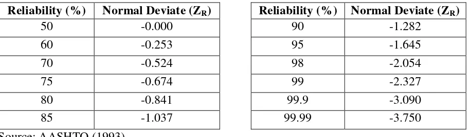
Reliability of performance-design controlled with reliability factor (FR) which is multiplied with the traffic estimates (w18) over the design life to obtain performance predictions (W18). For a given level of reliability, the reliability factor (FR) is a function of the overall standard deviation (So), which takes into account the possibility of a variety of traffic estimates (w18) and performance estimates (W18) given. In flexible pavement design equation, the level of reliability accommodated with the parameters of the standard normal deviation (ZR). Table 2.3 shows values of ZR for certain service level.
Table 2.3: Standard Normal Deviation for Certain Reliability Service
Application of the concept of reliability should consider the following steps:
1. Define the functional classification of roads and determine whether it is an urban road or inter-urban (rural) road.
2. Select the level of reliability from interval that given in Table 2.2.
3. Standard normal deviation of the corresponding reliability can be seen in Table 2.3.
b. Overall Standard Deviation (So)
Overall standard deviation is a combination of standard error of traffic prediction and road performance. This variable measures how far the probability of traffic prediction and road performance deviate from the design. For instance, it is predicted that the number of traffic is 2.000.000 ESAL for the next 20 year, however, in fact, there are 2.500.000 vehicles in that period. The larger the deviation is, the higher the value of So will be. For flexible pavement, the value of So is 0.35 – 0.40 (AASHTO, 1993).
2.3.5 Subgrade Bearing Capacity MR
The MR of the subgrade soil seen in the equation (2.1) has been adjusted to take into account for seasonal changes, and is termed as the effective MR. This is done to take into
account for differences in testing procedures from the road test and the current testing method using fallingweight deflectometer (FWD). At the road test, Screw driven laboratory devices were used to determine the soil stiffness. Due to slow response time of such devices, the apparent stiffness of the soil was very low (around 3,000 psi). With the much more rapid loading of FWD testing, the moduli are typically around three times higher, and therefore the moduli are divided by three to arrive at similar numbers to those used at the road test (Dives2009).
MR measurement should be conducted routinely during a year to observe the relative
The layer thickness produced from SN equation does not have a single unique solution, i.e. there are many combination of layer thickness of the flexible pavement layers. It is necessary to consider their cost effectiveness along with the construction and maintenance constraints in order to avoid the possibility of producing an impractical design from a cost effective view. If the ratio of costs for layer 1 to layer 2 is less than the corresponding ratio of layer coefficients, then the optimum economical design is one where the minimum base thickness is used since it is generally impractical and uneconomical to place surface, base or subbase courses of less than some minimum thickness (AASHTO, 1993)
a. Drainage condition
Table 2.4: The Definition of Drainage Quality shows drainage coefficient value (m) which is a function of drainage quality and percentage of time in a year pavement structure will be affected by water content that close to saturated.
Table 2.5: Drainage Coefficient (m)
Remarks: *) depends on annual average rainfall and drainage condition at the road structure. Source: AASHTO (1993)
b. Coefficient of Relative Strength
This guideline introduces a correlation between relative strength coefficient with mechanistic value, namely modulus resilient. Based on the type and function of pavement layer material, estimation of relative strength coefficient is grouped into 5 categories, namely asphalt concrete, granular base, granular subbase, cement-treated base (CTB), and asphalt-treated base (ATB) (AASTHO, 1993).
Quality of drainage
(1) Asphalt Concrete Surface Course
Figure 2.3 show the graphic that used to estimating the relative strength coefficient of Asphalt Concrete Surface Course (a1) that has dense gradation based on Modulus Elasticity (EAC) at 68oF temperature (AASTHO 4123). Although the modulus of asphalt concrete is higher, stiffer, and more resistant against deflection, but it is more susceptible to fatigue crack (AASHTO, 1993).
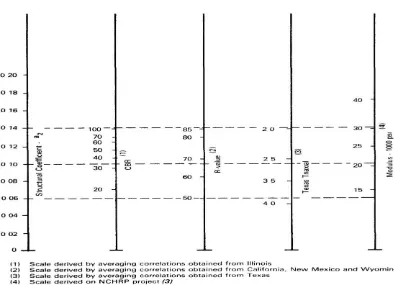
(2) Granular Base Layer
Relative strength coefficient (a2) can be estimated by using Figure 2.4. (3) Granular Subbase Layer
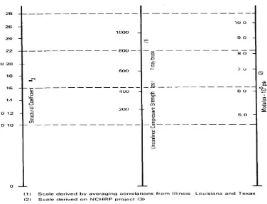
Relative strength coefficient (a3) can be estimated by using Figure 2.5. (4) Cement-Treated Base (CTB)
Figure 2.6shows the graph that can be used to estimating relative strength coefficient, a2 for cement-treated base (CTB).
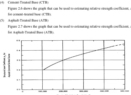
(5) Asphalt-Treated Base (ATB)
Figure 2.7 shows the graph that can be used to estimating relative strength coefficient, a2 for Asphalt-Treated Base (ATB).
Figure2.6: Variation of Relative Strength Coefficient of Cement-Treated Base (a2)
2.3.7 Determination of Structural Number
Figure 2.2shows the nomograph to determine Structure Number. The nomograph can be used if all following parameters are available:
1. Traffic estimation in the future (W18) at the end of design life 2. Level of reliability (R)
3. Standard deviation (So)
4. Effective resilient modulus of subgrade material (MR) 5. Loss of serviceability (∆PSI = po - pt)
The calculation of pavement thickness in this guideline is based on the relative strength of each pavement layers, using formula as shown in Equation (2.1).
2.4 Single Axle Load Equivalency Factor (LEFs)
Using the fourth-power relationship found at the AASHO Road Test, equations were derived to relate axle loading to pavement damage. Replicate cross sections were constructed in different test loops to apply varying repeated axle loads on the same pavement structure. This allowed the researchers at the road test to view the damage caused by heavier axles, and create mathematical relationships based upon that damage. The resulting pavement damage was quantified using single axle load equivalency factors (LEFs), which are used to find the number of ESALs. An LEF is used to describe the damage done by an axle per pass relative to the damage done by a standard axle per pass. This standard axle is typically an 18-kip single axle, as defined in the road test. From the AASHO Road Test results, the LEF can be expressed in the following form according to Huang (2004). The EALF can be expressed in the following form according to Huang (2004):
(2.11)
SN of 5 for the determination of 18-kip single axle equivalence factors will normally give results that are sufficiently accurate for design purposes. Even though the final design may be somewhat different, this assumption will usually result in an over estimation of 18-kip equivalent single axle when more accurate results are desired and the computed design is appreciably different (1 inch of asphalt concrete) from the assumed value. A new value should be assumed and the design 18–kip ESAL traffic (W18) recomputed. The procedure should be continued until the assumed and computed values are sufficiently close (AASHTO, 1993).
2.5 Previous of Studies
Several previous studies on road damage that have been done by previous researchers are as follows.
1. Rahim (2000). The analysis conducted was to calculate cost loss of road pavement distress resulted from overloading and therefore the amount of loss cost the overload car users shall bear can be determind. Overload heavy vehicle causes road pavement structure distress and service lifetime decreasing during design life time . The presence of overloading is indicated by the width area of rutting which is more than 60% of total road structural distress per km and by maximum axle load (MAL) of the heavy vehicle which is larger than the standard MAL. The cost loss of road pavement distress due to overloading is calculated based on damage factor (DF) and deficit design life (DDL). The loss of the overload car user shall bear 60% of total DFC (damage factor cost) and DDLC (deficit design life cost). Rahim (2000) was considering that not all pavement structural distresses are absolutely caused by overloading freight transport.
2. Koesdarwanto (2004) evaluated the service life of flexible pavement as a function of overloaded vehicles. Koesdarwanto concluded that the overloaded vehicles could decrease service life of road pavement from 5 years to 8 years.
CHAPTER 3 METHODOLOGY
3.1 Overview
The methodology is a flow chart or structural steps to solve a problem with a scientific approach. Every completed step should be evaluated with great accuracy in order to produce results as expected.
3.2 Research Methodology
In general, this research is conducted in several stages, as seen in Figure 3.1. The detail of each stage is presented in the following sections.
3.2.1 Preparation Stage
Preparatory work includes activities such as literature review of previous related studies in road sector, review the theories about the design of road pavement, and develop a methodology of the research.
3.2.2 Data Collection
At this stage, all data related to this research were collected. This study only employed secondary data, which is consisted of
• Traffic volume
• Vehicle weight that overloading was occurred (especially trucks).
• Soil strength in terms of California Bearing Ratio (CBR).
• Thickness of existing pavement layers in Demak-Trengguli road section.
Figure 3.1: Methodology of This Study
3.2.3 Data Analysis
The secondary data obtained was analyzed on the basis of literature review and theories that had been learned. They are: Traffic volume and load data Roughness, MR and CBR
Evaluation Evaluation
To know the existing physical condition, such as IRI, CBR, ADT obtained from Bina Marga.
(2) Design condition
Calculation of layer thickness using existing data was performed in order to know the differences between thickness of existing and design layers in Demak-Trengguli road section. The steps of calculation consist of:
a. Determine the volume of traffic (design ADT) from survey data b. Calculate vehicle damage factor (VDF)
c. Calculate cumulative equivalent single axle load (CESAL) using actual VDF based upon design and existing condition.
d. Calculate pavement thickness based upon design and existing CBR and IRI. e. Calculate pavement service life for design and existing condition.
3.2.4 Evaluation
The purpose of this stage is to evaluate the results obtained, by following the procedure: a. Determine of the thickness difference between normal and overloaded conditions. b. Determine the reduction of pavement service life for normal and overloaded conditions
to know the rest of service life of Demak-Trengguli road section.
3.2.5 Conclusion
CHAPTER 4
RESULTS AND ANALYSIS
4.1 Analysis of Traffic Data
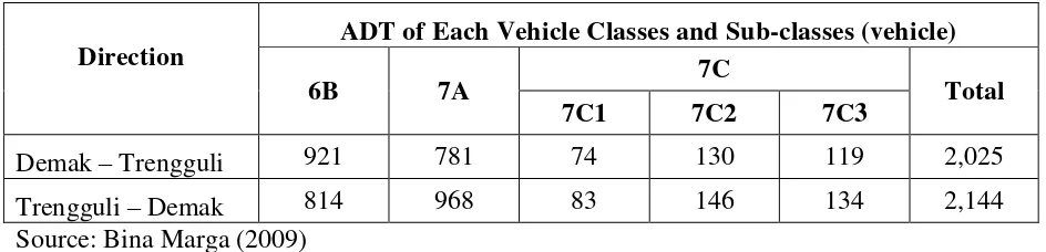
In this study, analysis of traffic data in the means of calculating average daily traffic (ADT) was performed by summing all groups of vehicles for the entire survey period 24-hours a day and then divided on how many days to collect the 24-hour data. The data survey period was 5 days for each direction. However, the full-set data, i.e. 24-hour traffic data, available in this study was only 3 days. Therefore, all traffic analyses in this study were based upon these 3-day traffic data. According to Bina Marga standards (2009), vehicles could be categorized into 7 classes, however, only three classes of vehicles categorized as truck-type (heavy vehicle) that were considered in this study, in accordance with 1993 AASHTO Design Guide requirement. They are vehicle-class of 6B for 2-axis trailer, 7A for 3-axis trailer and 7C for more than 3-axis trailer. Vehicle-class 7C consists of three sub-classes; they are 7C1 for 4-axle trailer, 7C2 for 5-axle trailer and 7C3 for 6-axle trailer. The ADT of heavy vehicles for both directions for three-day survey is as shown in Table 4.1 below.
Table 4.1: ADT for Heavy Vehicles
Direction
ADT of Each Vehicle Classes and Sub-classes (vehicle)
4.2 Determination of Vehicle Damage Factor (VDF)
VDF or axle load equivalency factor (LEF or E) of each heavy vehicle was determined using 1993 AASHTO Design Guide procedure, as follows.
1. The axle load unit was converted from ton to kips and the type of the axle load was determined whether it is single, tandem or triple axles.
2. VDF or E was determined by correlating the axle load (see the first column of Tables 4.2, 4.3 and 4.4 for single, tandem and triple axles, respectively) and its corresponding VDF value (see the rest columns of the tables). The selected VDF was the value under pavement structural number (SN) equals to 5, as recommended by 1993 AASHTO Design Guide. In this study, all axle load equivalency factor tables were associated with terminal serviceability (pt) equals to 2.
3. The VDF of front and rear axles for every type of heavy vehicle were calculated based upon the configuration specification defined by Bina Marga (2009)
4. The VDF for each heavy vehicle was determined by summing its corresponding front and rear axles. Then, the total VDF for each type of heavy vehicle could be calculated. The results for VDF for each type of heavy vehicle are shown in Table 4.5.
Source AASHTO (1993)
Table 4.5: Total VDF for Each Type of Heavy Vehicle Used in This Study
As seen in Table 4.5, the total VDF of Demak – Trengguli direction is higher than the opposite direction. The deviation of VDF is mainly contributed by VDF of classes 6B, 7C1 and 7C3.
4.3 Calculation of Traffic Load
The calculation of traffic load W18 in equivalent standard axle load (ESAL) should be based on the actual VDF and ADT. AASHTO Design Guide gives the following formula to determine the traffic load for design lane (W18).
x x GRi
x 365Ei = axle load equivalency factor or vehicle damage factor (VDF) for axle load i;
GRi = annual growth rate (depends on traffic growth rate, g, in percent; and service life, n, in year) axle load i;
Road section Demak – Trengguli or Trengguli - Demak is a four-lane two- direction divided (4/2 D) road, therefore, in this case, DD and DL equal to 1 and 0.8, respectively. The traffic load on Demak – Trengguli or Trengguli – Demak road section was assumed to increase 6% per anuum and the road could serve traffic load for the next 10 years. Based on this assumption, the traffic load W18 on Demak – Trengguli and Trengguli – Demak in two conditions, i.e. standard (as designed) and overloaded conditions, are depicted in the following table.
Table 4.6: Traffic load (as designed and overloaded condition)
Direction W18 (in million ESAL)
As Designed Overloaded
Demak – Trengguli 19.542 100.850
Trengguli – Demak 20.715 40.380
Table 4.6 shows that there is no different on traffic load for both directions in standard condition, but in overloaded condition, traffic load of Demak -Trengguli direction is 2.5 higher than opposite direction. This is because the significant deviation of the VDF in Demak-Trengguli direction (see table 4.5), although the ADT of Demak-Trengguli was lower than the opposite direction.
4.4 Reduction of Pavement Service Life
Two impacts of overloaded heavy vehicles on road pavement that took into account in this study, namely, reduction of pavement service life and the need of structural capacity improvement in terms of layer thickness.
The reduction of service life could be indicated by the deviation of the pavement service life due to different magnitude of traffic load that have to withstand by the pavement structure. To calculate the reduction of service life, a relationship between traffic load and service life is able to be developed by using the 1993 AASHTO Design Guide equation as follows.
in which W18 is the predicted traffic load (in ESAL); w18 is the traffic load in basic year (in ESAL); the other parameter is as previously defined. The traffic loads in basic year for both conditions (standard and overloaded) are as shown in Table 4.6. These values and Equation (4.1) were used to plot predicted traffic load curves in Figures 4.1 and 4.2 for Demak – Trengguli and Trengguli – Demak directions, respectively.
Figure 4.1: Service Relationship between Traffic Load and Service Life on Standard and Overloaded Conditions (Demak – Trengguli Direction)
Figure 4.2: Relationship between Traffic Load and Service Life on Standard and Overloaded Conditions (Trengguli – Demak Direction)
As shown in the figures, the curves have the following equations.
Y = 1.044X2 + 14.25X + 9.73 (4.2) Y = 4.219X2 + 57.62X + 39.32 (4.3)
for standard and overloaded conditions (Demak – Trengguli direction), respectively. And,
Y=1.136X2 + 16.62X + 29.96 (4.4) Y=1.869X2 + 27.34X + 49.28 (4.5)
for standard and overloaded conditions (Trengguli – Demak direction), respectively.
Using the equations, the reduction of service life due to overloaded condition can be determined, as shown in Table 4.7 below.
Table 4.7: Relationship between Traffic Load and Service Life
No of.year
Traffic Load of Demak – Trengguli (million ESAL)
Traffic Load of Trengguli – Demak (million ESAL)
For example, the standard traffic load of Demak – Trengguli in 10 years is 257,566,000 ESAL, but this number in overloaded condition is reached in 3.077 years. This means that there is about 7 years reduction of service life because of overloaded heavy vehicles. In the same manner, the standard traffic load of Trangguli – Demak in 10 years will be reached in overloaded condition after 6.573 years, so that the reduction of service life due to overloading is about 4 years. It means that the overloaded condition could reduce the service life about 4 times and 2 times for
4.6 Calculation of Structural Capacity
To calculate the structural capacity of road pavement, as represented by structural number (SN), it is necessary to determine several parameters as follow.
4.5.1 Loss of Serviceability (∆PSI)
The loss of serviceability can be determined by following the procedure below.
a. Average IRI was calculated from the existing data for 8 station of each direction. The IRI for all stations can be seen in Tables 4.8 and 4.9 below.
Table 4.8: Loss of Serviceability for Demak – Trengguli Direction
Station IRI (m/km) SV X po ∆PSI
Table 4.9: Loss of Serviceability for Trengguli – Demak Direction
Station IRI (m/km) SV X po ∆PSI
b. PSI (in this case, PSI was referred to initial serviceability, po) can be obtained by using the relationship between PSI and IRI, as follows.
where:
(2.7)
(2.8)
c. Loss of serviceability could be calculated using the following equation.
∆PSI = po- pt (4.6)
where po is initial serviceability index (calculated by using equation 4.8 above) and pt is terminal serviceability index. In this study, the terminal serviceability used equals to 2. The use of pt = 2 is caused by the minimum terminal serviceability provided by AASHTO’s axle load equivalency factors tables equals to 2. The calculation result ∆PSI for two directions are depicted in Table 4.8 and 4.9.
In Tables 4.8 and 4.9, there are road sections having high IRI values that cause the initial serviceability (po) is less than terminal serviceability (pt). To overcome this problem, all initial serviceability; that was less than two, was equated to two.
4.5.2Resilient modulus (MR)
The value of resilient modulus could be measured according to AASHTO procedure or based on relationship with other parameter, such as California Bearing Ratio (CBR). This relationship is represented by the following equation.
MR (psi) = 1500 x CBR (2.9)
Table 4.10: Modulus Resilient of Subgrade
4.5.3 Calculation of Structural Number (SN) and Layer Thickness (D)
The structural capacity of road structure, represented by SN, is determined by the following procedure.
a. SN3, SN2 and SN1 were determined based on resilient modulus of subgrade, subbase and base layer, respectively, using AASHTO design thickness equation (see equation 2.1) The three values of SN were calculated using data from the following input parameter which is corresponding with standard and overloaded conditions: traffic load, W18 (see Table 4.7), and loss serviceability (PSI) (see Tables 4.8 and 4.9). Other parameters, R or ZR and So, were assumed to be similar for the two conditions, that are, R = 90% or ZR = -1.282 and So = 0.35.
c. The layer thickness was calculated using the following equations rehabilitation work, it is common not to disturb the existing layers and add another layer on top of existing surface layer, called as overlay. The thickness of overlay can be obtained by subtracting the total thickness of surface layer (D1 in Tables 4.12 and 4.14) with the thickness of existing surface layer (D1 in Tables 4.11 and 4.13). The example of thickness calculation can be seen in Appendix D.
Table 4.12: SN and Layer Thickness of Road of Demak - Trengguli Direction
Table 4.13: SN and Layer Thickness of Road of Trengguli - Demak Direction (Standard Condition)
It can be seen from the tables above that there are significant differences between the structural number and thickness of each layer for two conditions (standard and overloaded). The summary of SN and thickness calculation is shown in Table 4.15 below.
Table 4.15: Summary of SN and Thickness Calculation Average SN3 Average D1 (in.)
From Table 4.15, it can be seen that there is a significant difference between structural number SN3 and thickness of surface layer (D1) for two conditions, i.e. standard load and overloaded
conditions. It is interesting to know that the difference between the structural number and surface layer thickness for two directions was not too much, although the traffic load of Demak-Trengguli direction was 2.5 times higher than that of opposite direction. This could be contributed by the ability of the pavement structure of Demak-Trengguli direction to withstand load was higher than that of the opposite direction (see Tables 4.8 and 4.9).
CHAPTER 5
CONCLUSIONS AND RECOMMENDATIONS
5.1 Conclusions
From the analysis of this study on "Identification of Damage due overloading on Demak-Treangguli Road”, it can be concluded that:
a. The average daily traffic (ADT) of heavy vehicle for Demak-Trengguli and Trengguli-Demak directions are 2,025 and 2,144 vehicles/day, respectively. It means that the ADT for Trengguli- Demak direction is more than the opposite direction
b. The average of vehicle damage factor VDF for Demak-Trengguli and Trengguli-Demak directions are 98.10 and 46.48 ESAL, respectively. It means that the heavy vehicles on Demak-Trengguli direction bring heavier goods than that of the opposite direction.
c. The equivalent standard axle load of heavy vehicle for Demak-Trengguli and Trengguli-Demak directions are about 100.85 and 40.38 million.ESAL, respectively.
d. Because of overloaded heavy vehicles, the service of life Demak-Trengguli direction is reducing from the original design 10 to 3 years, so that there is service life loss of 7 years. The similar condition is also encountered in the opposite direction Trengguli-Demak direction, where the service life reduces from 10 to 6.5 years, showing the service life loss of 4 years.
e. From the comparison of service life loss between both directions, it is very clear that the pavement layers of Demak-Trengguli direction needs more overlay thickness than that of the opposite direction.
5.2 Recommendations
From the conclusions mentioned above, there is a given suggestion to be considered or perhaps to be followed by some improvements, namely they are:
2. It is necessary to evaluate the condition of the design with reality at the beginning of the design life.
3. It is recommended that all data should be measured in the same day
REFERENCES
AASHTO (1993), AASHTO Guide for Design of Pavement Structures, Washington, D.C
Badan Litbang Departemen PU (2004), Laporan Ringkas kondisi Ruas Jalan Lintas Timur
Sumatera dan Ruas Jalan Pantai Utara Jawa, Jakarta (in Bahasa Indonesia).
Sulisty, B.S. and Handayani, C. (2002), The effect of heavy vehicle’s overloading to the
pavement damage/service life, Thesis, Department of Civil Engineering University of
Diponegoro Semarang, Indonesia.
Hudson, W.R., Monismith, C.L., Dougan, C.E., and Visser, W. (2003), Use Performance
Management System Data for Monitoring Performance: Example with Superpave,
TransportationResearch Record 1853, TRB, Washington D.C.
Al-Omari, B. and Darter, M.I. (1994), Relationships between International Roughness Index and
Present Serviceability Rating. Transportation Research Record 1435, Transportation,
Research Board, Washington, D.C.
Chen, H., Dere, Y., Sotelino E., and Archer G. (2002), Mid-Panel Cracking of Portland Cement
Concrete Pavements in Indiana, FHWA/IN/JTRP-2001/14, Final Report .
Davids, W.G. (2000), Foundation Modeling for Jointed Concrete Pavement, Journal of Transportation Research Record, 1730, Transportation Research Board, National Research Council, Washington D.C., pp 34-42.
Bina Marga (1997). Indonesia Highway Capacity Manual (MKJI), Departement of Public Works of Republic of Indonesia, Jakarta .
FHWA (2005), Long-Term Plan for Concrete Pavement Research and Technology - The
Concrete Pavement Road Map: Volume I, Federal Highway Administration, URL:
http://www.fhwa.dot.gov/pavement/pccp/pubs/05052/index.cfm, Publication number: FHWAHRT-05-0520, Accessed on September
Gillespie, T.D., Karamihas, S.M, Cebon, D., Sayers, M.W., Nasim, M.A., Hansen, W., and N. Ehsan (1993), Effects of Heavy Vehicle Characteristics on Pavement Response and
Performance, National Cooperative Highway Research Program Report 353,
Hall, K.T., and Munoz, C.E.C. (1999), Estimation of Present Serviceability Index from
International Roughness Index. Transportation Research Record 1655, Transportation
Research Board, Washington, D.C. 1999.
HRB (1962), The AASHO Road Test. Special Reports 61A, 61C, 61E. Highway Research Board. Holman, F. (1990) Guidelines for Flexible Pavement Design in Alabama. Alabama Department
of Transportation,
Huang, Y.H. (2004), Pavement Analysis and Design. 2nd ed. New Jersey: Prentice Hall
Koesdarwanto (2004), Evaluation of Flexible Pavement Service Life as a Function of
Overloaded Vehicles, Thesis, Surakarta Muhammadiyah University, Surakarta, Indonesia.
NCHRP (2004), Guide for Mechanistic-Empirical Design of New and Rehabilitated Pavement
Structures. Final Report for Project 1-37A, Part 1, 2 & 3, Chapter 4. National Cooperative
Highway Research Program, Transportation Research Board, National Research Council, Washington, D.C.
Rahim (2000), Analysis of Road Damage Due to Overloading on the Causeway in Eastern.
Sumatra .Riau Province. Thesis-S2, Master System and Transportation Engineering,
Gajahmada University (UGM), Yogyakarta.
Sayers, M.W. and S.M. Karamihas. (1998), The Little Book of Profilijng: Basic Information
About Measuring and Interpreting Road Profiles. University of Michigan.
Yu, H.T., Khazanovich, L., Darter, M.L., and Ardani, A. (1998), Analysis of concrete pavemenet
Responses to Tempertaure and Wheel Load Measured From Instrunmented Slabs. Journal
of Treansportation Reaserch Record, 1639, Transportation Research Board, National Research Council ,Washington ,D.C., pp.94-101
Zaghloul, S. and White, T.D. (1994), Guidelines for permitting overloads – Part 1: Effect of
overloaded vehicles on the Indiana highway network. FHWA/IN/JHRP-93–5. Purdue
Appendix A Traffic Data for Demak-Trengguli Direction
Result ADT 6,006 4,468 4,227 3,381 604 39 801 1,000 766 104 311
3 00 N 48 54 51 41 14 0 19 46 24 1 2
Result ADT 7,168 4,340 4,106 3,285 742 19 984 851 647 90 293
Day hour Direction type 1 type 2 type 3 type 4 type 5 A type 5 B type 6 A type 6 B type 7 A type 7B type 7 C
ADT 6,913 4,381 4,144 3,315 928 26 1,230 912 931 78 364
5 00 N 43 68 64 51 21 0 28 43 41 2 15
Result ADT 6,696 4,396 4,159 3,327 758 28 1,005 921 781 91 323
Appendix A Traffic Data for Trengguli- Demak Direction
ADT 7,602 4,094 3,873 3,098 595 39 788 918 990 153 370
3 00 O 48 54 51 41 14 1 19 41 31 4 3
ADT 7,168 4,340 4,106 3,285 742 36 984 731 815 128 325
Day hour Direction type 1 type 2 type 3 type 4 type 5 A type 5 B type 6 A type 6 B type 7 A type 7B type 7 C
Result ADT 6,913 4,381 4,144 3,315 928 43 1,230 792 1,099 114 392
5 00 O 43 68 64 51 21 1 28 38 48 3 16
Result ADT 2,670 1,940 1,835 1,468 464 17 614 385 471 71 144
Appendix B for International Roughness’ Index Normal Demak-Trengguli
Normal (Demak-Trengguli)
SECTION ID SUBDISTANCE TOTALDISTANCE IRI EVENT GOOD MUDIUM POOR VERY POOR
Normal (Demak-Trengguli)
SECTION IDSUBDISTANCE TOTALDISTANCE IRI EVENT GOOD MEDIUM POOR VERY POOR
14 0.3 4.802 3.5 0.1
TOTAL 6.246 RATA2 3.38 5.001 1.193 0.052 0
Normal (Demak-Trengguli)
SECTION IDSUBDISTANCE TOTALDISTANCE IRI EVENT GOOD MEDIUM POOR VERY POOR
Normal (Demak-Trengguli)
SECTION IDSUBDISTANCE TOTALDISTANCE IRI EVENT GOOD MEDIUM POOR VERY POOR
Appendix B for International Roughness’ Index Opposite Trengguli -Demak opposite (trengguli-Demak)
SECTION IDSUBDISTANCE TOTALDISTANCE IRI EVENT GOOD MEDIUM POOR VERY POOR
APPENDIX D
EXAMPLES OF CALCULATION
D.1 Calculation of Vehicle Damage Factor (VDF)
In this section, the calculation of VDF for 6B-class truck is presented. In this study, the calculation of VDF was performed based on axle load equivalency factor (LEF) tables with pt = 2, i.e. Tables 4.2-4.4. The 6B-class truck has one single axle on the front and rear. The detail calculation is as follows
- Axle load on the front : 4,965 ton
- Axle load on the rear : 5,193 ton
To enable using the axle load in 1994 AASHTO axle load equivalency factor (LEF) tables (see Tables 4.2-4.4), it is necessary to change the unit of the axle load parameter, from ton to kips, by multiplying the value of axle load (in ton) with a constant 0.002206. This result in 10.95 and 11.46 kips for front and rear axle loads, respectively. Since there is only one type of axle load in this calculation, that is, single axle load, therefore only Table 4.2 was used.
In this table, it not possible to find axle load equals to 10.95 and 11.46 kips in the first column; therefore an interpolation is required by interpolating the axle load values between 10.95 and 11.46 kips, and its corresponding LEF values (under structural number SN = 5) 0.079 and 0.174 ESAL, respectively. The following interpolation equation was used in this study.
Y (ESAL) = (X-X2)/(X1-X2)*(Y1-Y2)+Y2 (D.1)
where:
X1 = the first axle load value (kips) X2 = the second axle load value (kips)
Using Equation (D.1), the LEF that corresponding with axle load equals to 10.95 kips is as follows.
Y = (10.95-12)/(10-12)*(0.079-0.174)+0.0174 = 0.12 ESAL
Using the same equation, the LEF that corresponding with axle load equals to 11.46 kips is 0.15 ESAL. The VDF for 6B-class truck is 0.12 + 0.15 = 0.27 ESAL.
D.2 Calculation of Layer Thicknesses
The calculation of layer thickness is carried out by using the equations below.
SN3 = a1D1 + a2D2 m2 + a3D3 m3 (4.7a)
In order to calculate overlay thickness, the following equation was used.
DOL= (SN3- (a2 x D2 x m2 + a3 x D3 x m3)/a1 (D.2)
Using the previous data, the overlay thickness DOL can be calculated as follows.