*Correspondence address: Department of Economics, University of Girona, Avda. Lluis SantaloH, 17071 Girona, Spain. Fax:#34/972/418032; e-mail: [email protected].
24 (2000) 143}163
The dynamics of spatial pollution:
The case of phosphorus runo!
from agricultural land
Renan U. Goetz!,*, David Zilberman"
!Department of Economics, University of Girona, Girona, Spain
"Department of Agricultural and Resource Economics, University of California, Berkeley, USA
Received 7 April 1997; accepted 7 October 1998
Abstract
The paper analyzes, based on a land classi"cation system, the optimal management of negative production externalities while taking into account the intertemporal and spatial aspects of the problem. To incorporate both aspects simultaneously, a two-stage modeling approach is proposed where the solution of the spatial problem ("rst stage) is optimized over time (second stage). As a result, it is possible to relate long-run and short-run supply and input demand functions. Attention is given to runo!s from agricul-tural land leading to the contamination of a water body, in particular, the one of phosphorus and the eutrophication of lakes. The employment of a land classi"cation system supports a full-information approach and allows to address the optimal manage-ment of mineral fertilizer and manure based on zonal taxes, zonal permits, and zonal standards which all vary over time. ( 2000 Elsevier Science B.V. All rights reserved.
JEL classixcation: C61; H23; Q24; Q25
Keywords: Space time-dependent optimal control; Pollution tax; Tradable phosphorus permits; Zoning
1. Introduction
Negative production externalities have been the concern of many economic studies. In the case where the pollutants accumulate over time, these studies were conducted within a dynamic framework. Besides the intertemporal aspect, the heterogeneity of space may be of prime consideration for the economic analysis of negative production externalities. Prominent negative externalities from agricultural production like the runo!of phosphorus (P) or the leaching of nitrogen (N) share the intertemporal and spatial aspect.
Hochman et al. (1977) analyzed the properties of optimal tax incentives schemes to control pollution in a spatial setting. Both aspects, time and space, were integrated in a modelling approach by Tomasi and Weise (1994). They focused their analysis on the optimal spatial allocation of agricultural land versus residential land over time. Yet, the agricultural land is often exogenously given, and the optimal management of nonpoint-source pollution needs to concentrate on the agricultural sector itself. Therefore, we de"ne agricultural activities, which allow us to address agricultural policy questions. We base our analysis on the full-information approach by employing a land classi"cation system which accounts for di!erences in environmental vulnerability of loca-tions and by considering improved monitoring technology to account for heterogeneity in residue (pollutant) generation (Khanna et al., 1998). In this way nonpoint-source pollution can be viewed as point-source pollution provided that an adequate monitoring technology and a classi"cation system exist. Most importantly, however, we present a modelling approach which consists of the simultaneous solution of the micro-level (agricultural production) and macro-level (aggregate supply and demand) over space and time. In particular, it allows us to derive relationships between long-run and short-run supply and input demand functions.
2. Environmental vulnerability and space
the water body (e.g., milligram of bioavailable P per liter) and take a"rst step in evaluating the potential damage.
To assess the environmental vulnerability of a location based on a land classi"cation system, this paper takes the P index, developed under the patron-age of the U.S. Department of Agriculture}The Natural Resources Conserva-tion Service}(Sharpley, 1995), as an example. The P index allows to assign each location within the catchment of the receiving water body the potential P load resulting from the cultivation of a particular crop with a given crop management practice while taking account of the particular characteristics of the water body. For the sake of concreteness, we consider the example of a lake. Phosphorus loadings of a lake above the sum of the permanent settling rate of P in the sediment and of the P losses through the out#ow of water lead to the euthropi-cation of a lake. This will result in excessive algae growth and a lack of dissolved oxygen (Spulber and Sabbaghi, 1994). As a result, the water quality of the lake declines which, in turn, reduces the biodiversity and recreational and commer-cial bene"ts of the lake. It also increases the costs for water treatment to provide drinking water or to supply water for manufacturing processes (Holmes, 1988; Spulber and Sabbaghi, 1994).
The P loading from agricultural land at a speci"c location within the water-shed depends on the water delivery ratio, the water body sensitivity, the land management, and on characteristics of the land, such as the soil P content and the erosion and runo!potential. The latter characteristics are incorporated in the P index by considering site-speci"c information such as soil texture, per-meability of the soil, rainfall, the length and gradient of the slope, the cultivated crop itself, and crop management and tillage practices. The factor soil P content includes available soil P and P absorption capacity. The water delivery ratio re#ects the share of P runo!transferred from the edge of the"eld to the lake, whereas the water body sensitivity accounts for factors such as the degree of surface mixing, the depth of the lake, water residence time, and the development of reducing conditions at the water sediment surface (Sharpley and Halvorson, 1994).
Let the P load for a given type of fertilizeri, associated with a particular crop, be denoted bya
i(o), whereorepresents a derived P index attributing a potential
P load to each location within the watershed, regardless of the type of fertilizer. Intuitively, one expects locations close to the tributaries of the lake or to the lake itself to have high potential P loads. Therefore, we associate a small o with a high P load. The economic loss resulting from the deterioration of the water quality of the lake is captured by the C(2) (twice continuously di!erentiable) damage functiond(s), wherespresents the concentration of bioavailable P in the lake. We propose thatd@(s)'0 anddA(s)50.
1For example, dairy, beef, swine, sheep and poultry manure has an average N : P ratio of 4.1 while the N : P requirements of major grain crops is 7.3.
application of plant protection agents. Analogous to the land classi"cation system with respect to P runo!, these systems would classify the land based on a variety of factors, where the measurement of the distance from a particular point of reference is only one among many other factors. In this paper we focus our analysis on the problem of P runo!s from agricultural land. However, to generalize our results, we also discuss the most important"ndings in the context of nitrogen leaching into the groundwater.
3. The economic model
Examples in the United States (Boggess et al., 1993) and Switzerland (Amt fuKr Umweltschutz, 1993) show that lakes are often euthropic where the number of large animal units per hectare is high. This can be explained by the fact that P runo!s from agricultural land, where manure has been applied, contains a high fraction of soluble phosphorus which is immediately available for biolo-gical uptake by the algaes. Moreover, manure application rates are based on the management of nitrogen, leading in most cases to an increase in soil P in excess of crop requirements. This is due to the generally lower ratio of N : P added in manure than what is taken up by crops1(Sharpley and Halvorson, 1994).
This situation suggests focus on the analysis on crop production and the stocking rate per hectares in order to"nd the optimal P concentration of the lake. For this purpose, let a
1(o) denote the P runo!s associated with the
application of mineral fertilizer u(o) anda
2(o) with the application of animal
manureb(o)oy(o), wherey(o) presents the number of large animal units,o'1 the amount of manure per large animal unit, andb(o)3[0, 1] the share of the available manure being applied. We assume for the case of P runo!s that
a
2(o)'a1(o),∀oas a result of the high P content and high bioavailability of the
manure compared to mineral fertilizer. Thus, the dynamics of the lake with respect toocan be stated as
sR"(a
1(o)u(o)#a2(o)b(o)oy(o))g(o), (1)
where a dot over the variables s or j, to be introduced later, indicates the operator d/do, andg(o) presents a density function. Furthermore, we assume that the entire agricultural land within the watershed is cultivated and is equal to one by an appropriate normalization procedure.
Eq. (1) can also be utilized to describe the dynamics of the concentration of nitrate in the groundwater, where a
associated with fertilizeri. Mineral fertilizer carries nitrogen in its mineral form, often in the form of nitrate. Thus, it is ready available by the plant, but the mineral fertilizer is also more suspectable to the leaching of nitrate than manure, where the nitrogen is predominately in its slow-releasing organic form. There-fore, the case of nitrate leaching suggests thata
2(o)(a1(o),∀o.
To complete the economic model, we like to introduce theC(2)crop produc-tion funcproduc-tion given byq(z) withq@'0 andqA(0, andz,u(o)#b(o)oy(o). Let the returns from livestock management be denoted byp
2y(o) and the associated C(2) cost function byc
3(y(o)), where we assume c@3'0 and cA3'0. The price
associated with the crop is denoted by p
1. Finally, we assume that a social
planner exists, who maximizes the present discounted net bene"ts from agricultural production within the watershed of the lake while taking ac-count of economic losses resulting from the accumulation of bioavailable P in the lake.
4. The management of phosphorus runo4s from agricultural land
4.1. Spatial and intertemporal aspects
To obtain an analytical solution more easily, we propose the framework of a two-stage optimal control problem. Basically, in the"rst stage we solve the spatial problem by determining the optimal trajectories ofu(o),b(o),y(o) ands(o) for everyo3[0,oN], whereoN indicates the upper limit of the P index. The value function<(o,uH(o),bH(o),yH(o);c), evaluated along the optimal path, indicated by the superscript *, re#ects the value of the solution for the optimal control problem of the"rst stage, given a parameter vectorc. In the second stage we solve theintertemporalallocation problem of the already optimized allocation problem with respect too. For this purpose, we employ<as a function of the parameterssoN ands0. Basically, the terminal value of the state variable in the"rst stage becomes the control variable in the second stage, and the initial value of the state variable in the"rst stage becomes the state variable in the second stage. The simultaneous solution of the two-stage optimal control problem yields the optimal trajectories ofu(t;o),b(t;o),y(t;o) ands(t;o).
2Given the inherent regional focus of the analysis, the product prices are not in#uenced by regional production decisions and thus they are taken as given. Therefore, the prices are also not in#uenced by the production of the externality, and we assume that the utility function of the consumers is quasilinear with respect to the traded goods and the externality. Thus, the optimal level of the externality is independent of the consumers'expenditures, and it is possible to derive a utility function which depends only from the externalitys(MasColell et al., 1995). To discuss the results of our model in a practical setting, we propose that the derived utility function can be represented by the damage functiond(s). Additionally, it is also assumed that there are no cost of public funds, and lump-sum transfers are available to redistribute income so that Pigouvian taxes are not distortion-ary (Sandmo, 1995). The assumptions made with respect to the quasilinearity of the utility function and the existence of costless public funds help to keep the model simple and allow us to concentrate our analysis on the optimal economic behavior and on the introduced approach of space and time-dependent optimal control.
4.2. The spatial decision problem
The solution of the social planner's decision problem2in the"rst stage is given by the value function<(s
oN,s0) de"ned as
<(s
0,soN), max u(o),b(o),y(o)
P
oN
0
[(p
1q(u(o)#b(o)oy(o))!c1u1(o)
!c
2((1!b(o))oy(o))#p2y(o)!c3(y(o)))g(o)] do!d(s(oN)) (P1)
subject to
sR(o)"(a
1(o)u(o)#a2(o)b(o)oy(o))g(o), s(0)"s
0, s(oN)"soN, b(o)3[0,1], u(o)50, y(o)50,
wheresoN indicates the resulting optimal terminal value ofs(oN), as a solution of
problem (P1) with no terminal constraint ons(oN). The parameterc1denotes the cost for mineral fertilizer, and c
2(w) is the C(2)cost function for shipping the
manure out o! the catchment area of the lake, with w,(1!b)oy(o), and c@
2'0,cA2'0. The terminal value function is given by the damage function devaluated at s(oN), the terminal value ofo, in other words, the damage that persists. The existence of the value function <(s
0,soN) can be concluded from
Theorem 11, p. 215 of Seierstad and Sydsvter (1987). To simplify notation, the argument o of the variables u,b,y,s,a
i,i"1, 2, and the variables
j,/
i, i"1, 2, 3, 4, to be introduced later, will be suppressed unless it is required
for an unambiguous notation.
Using Pontryagin's Maximum Principle, the Hamiltonian of the"rst stage H1 is given by
H1,(p
1q(u#boy)!c1u1!c2((1!b)oy)#p2y!c3(y) !j(a
Note the negative sign in front ofjto facilitate the interpretation of the costate variable. Taking account of the restrictions on the control variables leads to the Lagrangian L which reads as L,H1#/
1u#/2y#/3b#/4(1!b),
where/
i,i"1, 2, 3, 4, denotes the Lagrange multipliers. A solution of problem
(P1) has to satisfy the following necessary conditions, which are stated in accordance with Theorem 1, p. 276, and Theorem 3, p. 182, of Seierstad and Sydsvter (1987),
L
u"(p1q@(u#boy)!c1!ja1)g(o),
A
40; u"0
"0; u'0
B
(3)L
b"(p1q@(u#boy)#c@2((1!b)oy)!ja2)oyg(o),
A
40; b"0
"0; b3(0, 1)
50; b"1
B
(4)
L
y"(p2!c@2((1!b)oy)o!c@3(y)#(p1q@(u#boy)
#c@
2((1!b)oy)!ja2)bo)g(o),
A
40; y"0
"0; y'0
B
(5)jQ"#H1
s"0, (6)
sR"(a1u#a
2boy)g(o), s(0)"s0, s(oN)"soN. (7)
According to Corollary 2.1 of Feichtinger and Hartl (1986), there is no con-straint on j(oN) in form of a transversality condition. The value ofj(oN) is free. However, problem (P1) with no constraint on the terminal value on s(oN) requires, according to Proposition 2.1 of Feichtinger and Hartl (1986), the transversality condition
j(oN)"d@(s(oN)). (8)
Thus, it turns out that j(oN)"d@(s(oN)) since it re#ects the terminal value of jassociated with the unconstrained optimal spatial allocation. Additionally, the optimal values of the control variables and the Lagrange multipliers have to satisfy the Kuhn}Tucker conditions L
(i50,/i50 and /i
L
(i"0 for
i"1, 2, 3, 4. The constraint quali"cation will be satis"ed due to the linearity of the constraints inu,b, andy(Takayama, 1985).
Taking account of Eq. (8), Eq. (6) shows that
j(o)"d@(s(oN)). (9)
value is constant across space because the damage caused by agricultural production occurs outside the agricultural area.
In the following discussion of the necessary conditions, we assume an interior solution if not stated otherwise. The necessary condition (3) shows that the marginal product of fertilizer (mineral fertilizer and manure) has to equal the marginal costs of the application of the mineral fertilizer. Condition (4) suggests that the marginal product of fertilizer (mineral fertilizer and manure) and the foregone marginal costs of the shipment of manure have to equal the marginal cost of the application of the manure. Condition (5) indicates that the marginal return from livestock management has to equal the marginal cost of the shipment of manure and of the livestock management. The second term in condition (5), enclosed in brackets, is equal to zero according to condition (4). Additionally, condition (4) suggests that the entire animal manure (b"1) is applied on the "eld and no shipping takes place if the shadow cost are zero. Likewise fory'0, Eq. (5) indicates that the stock of animals increases when the shadow cost vanishes. The case where farmers face no shadow cost or only a fraction of it is widespread as noted by Kummert and Stumm (1992) and by the Committee on Long-Range Soil and Water Conservation Policy (1993).
The necessary conditions (3)}(5) also indicate how the variablesu,b,ywould respond in the short run to a decrease in transportation cost of the manure as a result of technological progress with respect to the cost function c
2(w).
Condition (3) shows that the entire amount of fertilizer is una!ected by a de-crease in transportation cost. Thus, we can conclude from Eq. (4) that (1!b)oy has to increase, implying that eitherbdecreases and/oryincreases. Finally, as noted above, Eq. (5) can be written asp2!c@
2((1!b)oy)o!c@3(y)"0. Since the
value ofc@
2((1!b)oy) is una!ected, we can conclude that technological progress
with respect to the transport of manure a!ects only the share of manure applied on the"eld but not the stock of animals.
4.3. The intertemporal decision problem
The value function<from the"rst stage is now utilized in theintertemporal optimal control problem of the second stage which is given by:
max
soN(t)
P
T0 <(s
oN(t),s0(t))e~dtdt#e~dTd(s0(¹)) (P2)
subject to
sR0(t)"soN(t)!(1#f)s
0(t), s0(0)"s0, soN(t)3S,
where from now on a dot over a variable indicates the operator d/dt. The initial value of the"rst stage problems
0now becomes the state variable in the second
stage depending ont. Hence,s
P in the lake;soN(t) is the sum ofs0(t) and the runo!of P from the agricultural land; d(s
0(¹)) the terminal value function;d'0, the social discount rate; and f, 0(f(1, the&decay rate'of bioavailable P due to its immobilization in the sediment or its#ow from the lake. The set Spresents the interval [0,sN]. One can think of sN as the saturation point of the bioavailable concentration of P derived from the biomass that can grow at the maximum in the lake. The argumenttof the controlsoN, state s0, and costate variableg, to be introduced later, are dropped to simplify notations whenever they are not required for an unambiguous notation. Hence, the Hamiltonian of the second stageH2 is given byH2,<(soN,s
0)!g(soN!(1#f)s0). Note again that a negative sign in front of
the costate variable g has been introduced so that the interpretation of g is facilitated. The necessary conditions for an interior solution (0(soN(sN) of problem (P2) are again stated in accordance with theorem 1 and 3 of Seierstad and Sydsvter (1987), and read as
H2
soN"<soN!g"0 N j(t;oN)"g(t), (10) gR"gd#H2
s0"g(1#d#f)#<s0 N gR"g(1#d#f)!j(t; 0), (11) sR0"soN!(1#f)s0, s0(0)"s0. (12)
Analogous to Eq. (8), the transversality condition is given by
g(¹)"d@(s
0(¹)). (13)
From the theory of optimal control, Theorem 9, p. 213, Seierstad and Sydsvter (1987), it is known that <
soN"j(oN) and <s
0"!j(0). Hence, the necessary
condition (10) shows that the shadow costs associated with the optimal solu-tions of problem (P1) and (P2) have to be identical for allt. Moreover, utilizing Eqs. (8) and (10), Eq. (11) can be written as gR(t)"d@(soN(t))(1#d#f)!j(t; 0). Employing Eq. (13) yields the particular solution of Eq. (11) given by
g(t)"d@(s
0(¹))!
P
Tt
d@(soN(v))(1#d#f)!j(v; 0) dv. (14)
Hence, Eqs. (8), (10) and (14) imply that
d@(soN(t))"d@(s0(¹))!
P
Tt
d@(soN(v))(1#d#f)!j(v; 0) dv. (15)
For t"¹, the stock variables soN(¹) ands
0(¹) of the problems (P1) and (P2),
respectively, have to be identical as it can be veri"ed by Eq. (15). Moreover, since (10) holds for allt, it implies thatjQ(t;oN)"dA(soN(t))sRoN"gR. Thus, along the
optimal path for t(¹ an increasing concentration of P in the lake, sRoN'0,
along the optimal path. Additionally, Eqs. (10) and (11) show that
jQ(t;oN)"j(t;oN)(1#d#f)!j(t; 0). Hence, the rate of change of the shadow cost is given by
jQ(t; oN )
j(t; oN )"d#f. (16)
Hence, the optimal rate of change of the shadow cost corresponds to the sum of the discount rate and the decay rate.
4.4. Implementation of a full-information environmental policy
Since farmers do not take the damage cost into account, the pollution of the lake will be higher than it is socially optimal. Within full-information, the socially optimal solution can be achieved by imposing the following taxes:
q
1(t,o)"j(t)a1(o) with respect to mineral fertilizer,q2(t,o)"j(t)a2(o)oy(o) with
respect to the share of the available manure applied, andq
3(t,o)"j(t)a2(o)b(o)o
with respect to large animal units. The introduction ofq
i(t,o),i"1, 2, 3, would
induce the farmer to choose the socially optimal value uH(o),bH(o), andyH(o), and he would face the necessary conditions (3)}(5) which warrant the socially optimal solution. For instance, ifa
1(o) were simply given by 1/(1#o) and, for
each location,ocould be interpreted in the case of P runo!s as the distance from the lake or, in the case of leaching of nitrate as the depth of the soil horizons above the aquifer, then the tax on mineral fertilizer would decrease with an increase in distance or in depth. Additionally, the tax on mineral fertilizer would also change over time according to the change inj(t). Yet, as indicated above, a measurement of distance from a particular point of reference is only one of many factors to be considered for the assessment of the environmental vulner-ability of a location. Therefore, the utilization of an index seems to be more appropriate. Most likely the index is not continuous but discrete. The imple-mentation of taxes, depending on time and space, based on a continuous classi"cation system would be very di$cult to administer. Hence, it is suggested that di!erent zones be introduced either according to a discrete index or according to speci"ed ranges for the parametero in the case of a continuous index.
In the case where the social planner knows neither the damage function nor the private production and cost functions, the socially optimal outcome could be achieved by the introduction of tradeable P permits. These permits would allow the owner to discharge a certain amount of bioavailable P into the lake. Depending ona
i(o),i"1, 2, and timet, these permits translate into a certain
5. Short-run analysis
5.1. Microlevel
After having analyzed the characteristics of the optimal path of the costate variables of the problems (P1) and (P2), we focus next on the impact of a variation in the costate variablejor in the parameters of the model on the optimal paths of the control variablesu,b,yof the"rst stage. As a result of the strict concavity of the functions q,!c
2 and !c3, the Jacobian matrix J,(L/L(u,b,y))(H1
u,H1b,H1y)@does not vanish over its entire domain. Thus,
Eqs. (3)}(5) can be solved globally and uniquely by using Theorem 6 in Gale and Nikaido( (1965) for u"uL(j;c),b"bK(j;c), and y"yL(j;c) where c,(p
1,p2,c1).
Thus, by the application of Cramer's rule, the following results can be obtained:
LuL
Lj" !1
detJo2y2[!a1cA2(w)cA3(y)!(a2!a1)p1qA(z)(c3A(y)#o2cA2(w))]~0, (17)
LbK
Lj" !1
detJ[(a2!a1)p1qA(z)oy(cA3(y)#cA2(w)o2(1!b))](0, (18)
LyL
Lj" !1
detJ[(a2!a1)p1qA(z)o2ycA2(w)](0, (19)
where detJ,cA
2(w)cA3(y)p1qA(z)o2y2(0. Hence, an increase in the shadow cost
is associated with a decrease in the stock of animals and in the amount of manure applied per hectare. Therefore, a higher share of the available manure is shipped out of the watershed. The reduction in manure applied however, may be o!set by an increase in the amount of mineral fertilizer applied per hectare. As Eq. (17) shows, LuL/Lj would be positive if a
1/(a2!a1)(!p1qA(z)(cA3(y)#
o2cA
2(w))/cA2(w)cA3(y). The term (cA3(y)#o2cA2(w))/c2A(w)cA3(y) is most likely greater
than 1 since its implication cA
3(y)/cA2(w)#o2'cA3(y) will be satis"ed under
normal conditions due to the high magnitude of o2. Therefore,
a
1/(a2!a1)(!p1qA(z) is a su$cient condition for an increase inuL resulting
from an increase in the shadow cost. Hence, a high product price of the crop, a strong curvature of the production function, or high P runo!s associated with the application of manure compared to the application of mineral fertilizer favor the application of mineral fertilizer.
In the context of leaching of nitrate into the groundwater, we noted above thata
1(o)'a2(o), thus reversing the order of the functionsai(o), i"1, 2 as in the
3Note that a comparative static analysis, which seemed to be more appropriate at"rst glance, cannot be conducted simply because a steady state of the "rst-stage problem, di!erent from
u"by"0, does not exist.
amount of manure applied on the"eld decreases while the amount of mineral fertilizer increases.
In order to analyze the e!ects of certain policies at the microlevel (the
"rst-stage problem) which a!ect the price of the crop, the cost of mineral fertilizer, or the returns of livestock management, we proceed with a compara-tive analysis based on pro"t-maximizing behavior. Additionally, we analyze the e!ects of a variation ina
1ora2on the spatial allocation of the control variables.
With respect to a decrease in a
1, one can think of subsurface placement of
mineral fertilizer, more precise determination of the required amount of mineral fertilizer according to the soil P content, and the implementation of P runo!
control strategies such as inter-cropping or not leaving the land fallow over winter. With respect to a decrease ina2, one can think of a more precise timing of the application of manure according to the requirement of the crop but also about the implementation of P runo!control strategies. Additionally, one can think of biotechnological progress leading, for example, to the development of a corn variety used as fodder where the P contained in the corn is absorbed to a higher extent by the livestock compared to previous corn varieties.
Based on this short-run microlevel analysis, we are able to determine the e!ects on the aggregate supply of the livestock, the aggregate demand for mineral fertilizer, for manure to be applied on the "eld, and for manure to be transported.3We recognize the fact that a comparative dynamic analysis might have been more appropriate. However, the results of a comparative analysis based on an approach, which was introduced into the economic literature by Oniki (1973), were not conclusive. Yet, as we show in the next section any optimal lake restoration strategy where the initial concentration of P in the lake is above the long-run optimal concentration of P in the lake requires thatj(t) as well assoN(t) decreases over time. Hence, we can take the optimal movement of jandsas given and concentrate our analysis on the necessary conditions which assure pro"t-maximizing behavior.
Looking at the variations in the parametersp
1andp2show that: LuL
Lp
1 "!1
detJcA2(w)cA3(y)q@(z)o2y2'0,
LuL
Lp
2 "!1
detJcA2(w)p1qA(z)o3y2(0, (20)
LbK
Lp
1
"0, LbK
Lp
2 " 1
LyL
Thus, we can conclude that the slope of the short-run demand function for mineral fertilizer is positively sloped with respect to the price of mineral fertilizer but negatively sloped with respect to the returns from livestock management. As expected, a rise inp
2will lead to an increase in the short-run supply of livestock
and to an increase in the short-run demand for manure applied on the"elds. However, an increase in the price of the crop has no e!ect on the short run supply of livestock and on the short-run demand for manure applied on the
"elds, since the shadow costs are constant in the short run and mineral fertilizer is a perfect substitute for manure and does not in#uence the return and cost of the livestock management. Appendix A contains the discussion on the e!ects of the variations in the parametersa
1,a2, andc1.
5.2. Macrolevel
The analysis at the microlevel helps to determine the aggregate e!ect on the short-run supply of livestock>, on the short-run demand for mineral fertilizer ;, and on the short-run demand for manure to be applied on the"eldB
aand to
be transportedB
t. The aggregate short run supply and input demand functions
are given by
1has the following e!ects
L>
An increase in the returns of livestock management a!ects the short-run aggregate supply and input demand functions in the following way:
L>
where the results of Eqs. (21) and (22) are used. An increase inp
2shows that the
short-run aggregate demand for mineral fertilizer decreases while the short-run aggregate demand for manure applied on the"elds increases and the short run aggregate demand for manure shipped out of the water catchment remains unchanged. Therefore, the short-run aggregate supply of livestock increases. The discussion of the e!ects of the variations in the P runo! coe$cients a
1 and a
2and the cost for mineral fertilizerc1is presented in Appendix B.
6. Long-run analysis
Finally we consider the case¹PRin order to study the comparative statics of the long-run solution of problem (P2). Therefore, we propose to reformulate problem (P2) in order to simplify the comparative static analysis. The revised version of problem (P2) is given by
max
0(t) in our previous notation, and the superscript = with
respect to a variable, denotes the evaluation of the variable at the steady-state value. We assume that the agricultural activities are allocated optimally over space. From this assumption, we conclude that there exists a one-to-one rela-tionship between P runo!s, denoted bysJ and monetary bene"ts presented by the function<I (sJ). Additionally, we assume that<I
will drop the argumenttof the variablessJ,s
0, and of the costate variablegunless
they are required for an unambiguous notation. The"rst-order conditions yield
<I
The transversality condition requires that lim
t?=g(t) is bounded (Caputo, 1992).
A linearization of the canonical system of the di!erential equations around the steady state values ofg,s
0results in
Since the trace of the Jacobian matrix
JI,
A
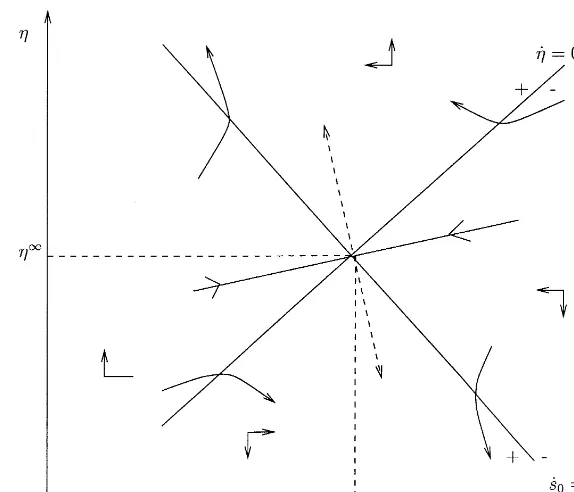
d one can conclude that the roots are real and have opposite signs. Hence, the steady-state equilibrium can be characterized locally by a saddle point.Additionally, the entries ofJI allow one to draw the phase diagram in the (s 0,g)
space. As Fig. 1 shows, the stable path leading to the steady state is upward sloping while the unstable path is downward sloping. Hence, along the optimal path, the shadow cost and the concentration of P in the lake are positively correlated. Therefore, any lake restoration policy, wheres
0's=0, can be
charac-terized by decreasing shadow cost and a decreasing concentration of P in the lake. By (10), we conclude thatj(t) also has to decrease along the optimal path. This particular link allows us to determine the short-run supply function of livestock and short-run input demand functions along the optimal path, and thus, deriving the optimal relationship between short-run and long-run supply and input demand functions. By Eqs. (17)}(19), we see that y and b has to increase whileumost likely has to decrease along the optimal path. Therefore, an optimal lake restoration policy, fors
0's=0, can be characterized by choosing
the stock of animals and the amount of manure to be applied on the"eld below their steady-state values while the amount of mineral fertilizer has to be chosen above its steady-state value. As time passes, the stocking rate and the amount of manure applied on the "eld increase while the amount of mineral fertilizer decreases until their steady-state values are reached.
Fig. 1. The phase diagram in the (s
0,g) space.
steady-state values, while the amount of mineral fertilizer is chosen below its steady-state value. Over time, the stocking rate and the amount of manure applied on the "eld decrease while the amount of mineral fertilizer increases until their steady-state values are reached. Hence, the reversal of the order of
a
i,i"1, 2 (the runo! coe$cient/leaching coe$cient) for a particular location
leads to the reversed optimal restoration policy.
6.1. Comparative statics
Next we analyze the variation in the parameters,dandf, on the steady-state equilibrium. GivengR"sR0"0, and detJI(0, we can solve Eqs. (30) and (31) for
g="gL=(d,f) ands=0"sL=0(d,f) by the application of the implicit function the-orem. Some calculations show that
LgL=
Ld"
1
detJI fg(0,
LsL=0 Ld"
1
detJI g<IsJsJ'0, (33)
LgL=
Lf"
1
detJI [fg#s0dA(s0)](0,
LsL=0 Lf"
1
detJI sJ(d#f)#
g <I
sJsJ
An increase in the social discount rate leads to an increase in the steady-state concentration of P in the lake whereas the steady-state shadow cost decreases. Intuitively, this can be explained by the fact that an increase in the social discount rate places a higher weight on the near future compared to the more distant future favoring the extension of agricultural activities with high P runo!s in the distant future. An increase in the decay rate decreases the steady-state shadow cost while the e!ect on the steady-state concentration of P in the lake is unclear. It remains an open question whether an increase in the decay rate leads to a decrease in the concentration of P. Maybe, as a result of an increase in the decay rate, the application of mineral fertilizer and/or manure increases and overcompensates the increase in the decay rate. By utilizing Eq. (10), the results additionally show thatjdecreases with an increase in the social discount rate or in the decay rate. Therefore, based on Eqs. (17)}(19) we can conclude that the long-run supply of livestock and the long-run demand for manure applied on the"eld rise with an increase in the social discount rate or the decay rate, while the long-run demand for mineral fertilizer may decrease or increase.
7. Summary and conclusions
This paper presents a full-information modelling approach for the socially optimal management of negative production externalities taking into account the aspects of time and space. In particular, we analyze the case of P runo!s into a lake and the leaching of nitrate into groundwater from agricultural land. The problem is solved in two stages. First, we determine the socially optimal spatial allocation of the agricultural production at the microlevel. Second, we solve for the socially optimal intertemporal allocation of the agricultural production at the macrolevel based upon the optimal spatial allocation. Hence, we can infer the optimal spatial allocation of the agricultural production from the optimal intertemporal allocation. To warrant the socially optimal outcome, we propose to introduce taxes on mineral fertilizer, on manure applied on the"elds, and on the stock of animals. The taxes re#ect the spatial and dynamic dimension of the considered production externality since one component of the tax varies over space and the other over time.
implementation of a zonal system of tradable permits, de"ned per kg discharge of bioavailable phosphorus into the lake. The permits cannot only be traded within a zone but also between zones. In this case the exchange relation of the permits is based upon the value of the P indices of the di!erent zones. According to the optimal water body restoration policy, the value of the permit changes over time, that is, the amount of admissible discharge in form of bioavailable phosphorus may decrease or increase over time.
When an improved monitoring technology at a!ordable costs is not available, the amount of mineral fertilizer or manure applied on the "eld cannot be observed or inferred by the regulator. In this case, the literature on asymmetric information related to nonpoint-source pollution (Tomasi et al., 1994) provides some solution.
This paper conducts an analysis for a region that is not signi"cant to a!ect the price of the output it produces. Further research should analyze the impact of regulation in cases where the industry is facing negatively sloped demand and the impact assessment should incorporate consumer surplus and price e!ects.
Acknowledgements
We would like to thank Anni Huhtula for her comments. Part of the work was completed while the"rst author was a$liated with the Swiss Federal Institute of Technology, Department of Agricultural Economics, ZuKrich, Switzerland.
Appendix A. Microlevel (variations in the parametersa1,a2andc 1)
We assumed with respect to the P runo! functions a
i(o), i"1, 2 that a
2(o)'a1(o),∀o. Hence, little information will be lost if we assume a
i(o),ai,i"1, 2. The functionsuL(j;c),bK(j;c) andyL(j;c) can equally be obtained
as before. However, the vectorcis now given byc"(p
1,p2,c1,a1,a2). A
vari-ation in the P runo!coe$cients yields
LuL
La 1
"!1
detJjo2y2[p1qA(z)(cA3(y)#o2cA2(w))!cA2(w)cA3(y)](0,
LuL La
2 " 1
detJjo2y2p1qA(z)[c3A(y)#o2cA2(w)]'0, (A.1)
LbK
La 1
" 1
detJjoyp1qA(z)[cA3(y)#(1!b)o2cA2(w)]'0,
LbK
La 2
"!1
LyL
The results show that a decrease ina
1has the opposite e!ect on the short-run
demand for mineral fertilizer, manure, and on the short-run supply of livestock than a decrease ina
2. Adecreaseina1, for example, due to better management
techniques with respect to the application of the mineral fertilizer, results in an increase in the short-run demand for mineral fertilizer while the short-run demand for manure applied on the"eld and the short-run supply of livestock decreases. Hence, the reduction of the P runo!coe$cient associated with the application of mineral fertilizer favors the substitution of manure by mineral fertilizer. Similar arguments, however, with the reversed sign hold for a decrease ina
2. Hence, biotechnological progress with respect to the P absorption
capa-city of the livestock shows that the short-run supply function of livestock is positively sloped and the short-run demand for mineral fertilizer is replaced by the short-run demand for manure applied on the"elds.
Finally, looking at a variation in the cost for mineral fertilizer results in
LuL
1yields the same results as a variation ina1, we present
only the signs of the short-run changes. An increase in the cost of mineral fertilizer leads to a decrease in the short-run demand for mineral fertilizer, while the short-run demand for manure and the short-run supply of livestock increase.
Appendix B. Macrolevel (variations in the parametersa
1,a2andc1)
A variation in the P runo! coe$cient with respect to the application of mineral fertilizer shows that
increases. The short-run aggregate demand for manure applied on the "eld, however, decreases. Hence, we see on the aggregate level in the short run a substitution of manure applied on the"eld by mineral fertilizer. Consequently, the short-run aggregate supply of livestock decreases, however, not su$ciently enough so that the short-run aggregate demand for manure shipped out of the watershed has to increase. With respect to a decrease in the P runo!coe$cient of manurea
2, we obtain, as expected, exactly the opposite results as discussed
for a decrease in the P runo!coe$cient for mineral fertilizer. As mentioned above, a variation inc
1on the microlevel yields the same results
as a variation ina
1. Therefore, we present only the signs of the variation in the
short-run aggregate supply and input demand functions.
L>
Lc
1
'0, L;
Lc
1
(0, LBa
Lc
1
'0, LBt
Lc
1
(0, (B.3)
The results show that the short-run aggregate supply function of livestock is positively sloped for an increase in the costs of mineral fertilizer. Additionally, we see on the aggregate level in the short run a substitution of mineral fertilizer by manure applied on the"eld. Since the short-run demand for manure to be shipped out of the watershed decreases with an increase inc
1, we can conclude
that the increase in the short-run supply of livestock is not su$ciently large to cover the higher short-run demand for manure applied on the"elds.
References
Amt fuKr Umweltschutz, 1993. Sanierung des Baldegger- und Hallwilersees und deren Einzugsgebiete, Situationsanalyse und Rechenschaftsbericht. Polizei- und Umweltschutzdepartement, Luzern. Boggess, W., Lacewell, R., Zilberman, D., 1993. Economics of water use in agriculture. In: Carlson,
G., Zilberman, D., Miranowski, J. (Eds.), Agricultural and Environmental Resource Economics, Chapter 8. Oxford University Press, New York.
Caputo, M., 1992. Dynamic Optimization and Comparative Dynamics, Lecture Notes AGE 254. University of California, Davis, CA.
Committee on Long-Range Soil and Water Conservation Policy, 1993. Phosphorus in the soil-crop system. In: Board on Agriculture, National Research Council ed., Soil and Water Quality}An Agenda for Agriculture, Chapter 7. National Academy Press, Washington.
Feichtinger, G., Hartl, R., 1986. Optimale Kontrolle oKkonomischer Prozesse. Walter de Gruyter, Berlin.
Gale, D., Nikaido(, H., 1965. The jacobian matrix and global univalence of mappings. Mathematische Annalen 15, 81}93.
Hochman, E., Pines, D., Zilberman, D., 1977. The e!ects of pollution taxation on the pattern of resource allocation: the downstream di!usion case. Quarterly Journal of Economics 91, 625}638. Holmes, T., 1988. The o!site impact of soil erosion on the water treatment industry. Land
Economics 64, 356}366.
Kummert, R., Stumm, W., 1992. GewaKsser als OGkosysteme, 3rd ed. Verlag der Fachvereine, ZuKrich. Mas-Colell, A., Whinston, M., Green, J., 1995. Microeconomic Theory. Oxford University Press,
New York.
Oniki, H., 1973. Comparative dynamics (sensitivity analysis) in optimal control theory. Journal of Economic Theory 6, 265}283.
Sandmo, A., 1995. Public"nance and the environment. In: Bovenberg, L., Cnossen, S. (Eds.), Public Economics and the Environment in an Imperfect World, Chapter 2. Kluwer Academic Publisher, Dordrecht.
Seierstad, A., Sydsvter, K., 1987. Optimal Control Theory with Economic Applications. North-Holland, Amsterdam.
Sharpley, A., 1995. Fate and transport of nutrients}phosphorus. Working paper 8, The United States Department of Agriculture, Agricultural Research Service, Durant, Oklahoma. Sharpley, A., Halvorson, A., 1994. The management of soil phosphorus availability and its impact on
surface water quality. In: Lal, R., Stewart, B. (Eds.), Soil Processes and Water Quality, Chapter 2. CRC Press, Boca Raton, FL.
Spulber, N., Sabbaghi, A., 1994. Economics of Water Resources: From Regulation to Privatization. Kluwer Academic Publisher, Dordrecht.
Takayama, A., 1985. Mathematical Economics, 2nd ed. Cambridge University Press, New York. Tomasi, T., Segerson, K., Braden, J., 1994. Issues in the design of incentive schemes for nonpoint
source pollution control. In: Dosi, C., Tomasi, T., (Eds.), Nonpoint Source Pollution Regulation: Issues and Analysis, Chapter 1. Kluwer Academic Publisher, Dordrecht.
Tomasi, T., Weise, A., 1994. Water pollution in a spatial model. In: Dosi, C., Tomasi, T. (Eds.), Nonpoint Source Pollution Regulation: Issues and Analysis, Chapter 7. Kluwer Academic Publisher, Dordrecht.