AN ALYSIS
Tools for recreation management in parks: the case of the
greater Yellowstone’s blue-ribbon fishery
Joe K erkvliet
a,*, Clifford N owell
baEconomics Department, Oregon S tate Uni6ersity, Cor6allis, OR 97331, US A bEconomics Department, W eber S tate Uni6ersity, Ogden, UT84088, US A
R eceived 21 April 1998; received in revised form 7 D ecember 1999; accepted 7 January 2000
Abstract
The recreationists who visit and enjoy the planet’s protected natural areas cause serious ecological damage to the very lands they enjoy. To maintain ecosystem integrity, park managers must increasingly focus on recreation management as a vital part of their jobs. M anagers agree on the importance of pursuing objectives using the least cost mix of tools. To make this choice wisely, the efficacy of various tools in influencing recreationists’ behavior must be assessed. R ecreation management is especially salient in many U S N ational Parks. F or example, wild Yellowstone R iver cutthroat trout inside Yellowstone N ational Park are caught an average of 9.7 times during the summer fishing season. Although managed as a catch and release fishery, up to 30% of these fish die each season at the hands of fly anglers. Anglers also cause streambank erosion, generate air, water and litter pollution, interact with wildlife and, for some, degrade the park’s scenic quality. In this paper we examine the extent to which the behavior of anglers in the greater Yellowstone ecosystem (G YE) is influenced by various management tools, including general and site-specific access fees, catch rates and regulations regarding the type and size of fish that can be killed. We also inquire whether anglers are likely to be self-regulating in that they self-select away from crowded fishing sites. U sing survey data from anglers at five popular fishing sites in the G YE, we estimate a two-part model of total site visitation. The two parts involve a discrete choice site selection decision for any given day and the choice of how many days to visit the G YE in a season. The product of the two decisions is total visitation to a site. We use the estimates to measure the impact of management tools on total anglers’ behavior. Our results indicate that anglers are averse to complicated regulations that target certain species and/or size of fish for releases, and prefer catch and release managed fisheries or those where all fish can be kept. We find that the total number of anglers’ visits is most strongly influenced by catch rates, followed by congestion levels and the cost of site-specific access. Increases in costs not specific to a site have little effect on anglers’ behavior. These results suggest that increases in the cost of season fishing permits or park entrance fees are not likely to reduce fishing pressure, but can be used to pursue revenue goals. In contrast, requiring anglers to pay a site-specific daily fee may be effective in managing anglers’ ecological impacts, but may be inconsistent with equity goals. © 2000 Elsevier Science B.V. All rights reserved.
www.elsevier.com/locate/ecolecon
* Corresponding author. Tel.: +1-541-7371482; fax: +1-541-7375917.
Keywords:R ecreation management; Yellowstone; Crowding
1. Introduction
N atural resource managers often confront the dual objectives of encouraging recreation while simultaneously preserving the ecosystems they manage. U nfortunately, human behavior often degrades natural processes. The recreationists who visit and enjoy the planet’s protected natural areas cause serious ecological damage to the very lands they enjoy (Alden, 1997). To maintain ecosystem integrity, park managers must increas-ingly focus on recreation management as a vital part of their jobs.
The choice of recreation management strategy requires that objectives be delineated and that the efficacy of the many tools at their disposal be evaluated (Alden, 1997). Choices are complicated by the fact that the use of some tools may retard progress toward certain objectives. Alden (1997) suggests that market mechanisms interfere with intra-generational equity goals and M cCarville et al. (1999) report that residents especially object to activity-specific fees. Conversely, a proposed recreation planning framework for U S national parks favors market methods over quantity con-straints because recreationists thereby retain more freedom of choice (G raefe et al., 1990, p. 7).
In spite of these differences, managers agree on the importance of pursuing objectives using the least cost mix of tools (G raefe et al., 1990; Alden, 1997). An important consideration in choosing the least cost mix of tools is the responses of recreationists to conditions created by their own behavior. We term these responses ‘self-regula-tion’. F or example, recreationists may self-regu-late by visiting an area less frequently after overuse degrades its amenities. H ere, self-regula-tion leads to reduced rates of visitaself-regula-tion and of degradation. Alternatively, crowds may signal a high quality recreational experience to potential visitors and result in more intensive use.
The implications of self-regulation may be de-sirable or undede-sirable, but managers will want to
understand its nature for three reasons. F irstly, self-regulation may be an inexpensive, low-profile alternative to more direct tools. Secondly, the stimuli for self-regulation, such as crowding or site degradation, directly impact recreation-based welfare. Thirdly, self-regulatory behavior is com-plex. Its impacts are not always be in the expected direction, and self-regulating recreationists may modify their activities in ways that adversely im-pact other parts of the ecosystem (K uss et al., 1990).1
R ecreation management is especially salient in many U S N ational Parks. Visitation has risen at an annual rate of 3.3% over the past decade. N ational Park Service (N PS) (1995) anticipates an additional 60 – 90 million visitors by the year 2000 (Wilkinson, 1995). F or years, the N ational Parks and Conservation Association has asked the N PS to address the problem of the human carrying capacity (Wilkinson, 1995).
Indeed, many question the validity of much of the human activity in the parks. R ecreational fishing is especially problematic. M cClanahan (1990, p. 5) writes, ‘Preservation will be difficult with the parks’ many external influences, but will be impossible if internal management allows recreation and resource use to supersede preserva-tion. The subjectivity of the fishing – hunting di-chotomy must be relinquished to a more objective management plan that preserves aquatic resources in the same manner as terrestrial species and ecosystems.’ The former associate editor of N ational Parks, Yvette La Pierre (1994, p. 38) writes ‘A growing number of people question the practice of fishing in the parks. Their argument is simple — the harvest of fish by angling is funda-mentally at odds with the mandate of the park
service to maintain natural ecosystems in an unimpaired condition’.
R esponding to such criticism and to some clear cases of over fishing, the N PS now manages nearly all waters in Yellowstone N ational Park (YN P) as catch-and-release fisheries. Still, some streams in and near YN P are heavily impacted by anglers. F or example, the wild, Yellowstone cut-throat trout (S almo clarki bou6ieri ) of the
Yellow-stone R iver inside YN P are caught an average 9.7 times during the 45-day summer season (Schill et al., 1986). Although managed as a catch-and-re-lease fishery, studies suggest that between 3 and 30% of the fish from these waters will die at anglers’ hands each season (H unsaker et al., 1970; Schill et al., 1986).
Besides this obvious impact, anglers cause streambank erosion, contribute to air, water and litter pollution, disturb wildlife and, for some, degrade the park’s scenic quality.2 YN P’s 1995
R esource M anagement Plan (1995; p.16) recog-nizes the ‘fundamental balancing act between pre-serving park resources and allowing human use. This issue particularly affects the park’s fisheries and back country programs, two of Yellowstone’s most popular visitor activities. H abituation and poaching of wildlife, disturbance of nesting birds, influx of exotic plant species, impacts to air and water quality, all relate to types and levels of human use’.
The N PS has an array of tools to attempt the ‘balancing act’ referred to above, including many that influence human behavior. They include edu-cation, various fees, queuing and the proscription of activities (G raefe et al., 1990). In the case of fisheries, the N PS may use regulations regarding the species and size of fish that may be kept. In some cases these tools may be effective; in others they are ineffective, expensive, unpopular, or in-consistent with other park management objectives (Alden, 1997).
A possible alternative or complement to these tools is a reliance on park users’ self-regulation. If park users, interacting with other visitors and the environment, behave so that the adverse impacts
of visitation are mitigated, then a laissez-faire approach is more appealing. One likely stimulus for self-regulation is crowding; that is, as park visitors become more numerous, recreationists will change their behavior by possibly visiting less often, changing the areas they visit, or changing their activities while visiting.
In this paper, we empirically examine the be-havior of anglers visiting the blue-ribbon trout fishery of the greater Yellowstone ecosystem (G YE), the bioregion that surrounds YN P. We use data obtained from a 1993 survey of anglers at five of the most popular G YE fishing sites. We address the efficacy of several management tools for influencing anglers’ behavior. These tools in-volve changes in anglers’ costs per trip, costs per day, site-specific costs, direct fisheries regulation regarding the harvesting allowed by species, size, or number and crowding’s contribution to an-glers’ self-regulation.
The paper is organized as follows. Section 2 discusses the modeling of anglers’ behavior. Sec-tion 3 briefly describes the angler survey we used to obtain data and presents the equations used for estimation. Section 4 discusses the statistical re-sults. Section 5 summarizes.
2. Anglers’ behavior and crowding-based self-regulation
F or a destination fishery such as the G YE, it is useful to consider anglers as making two choices. Anglers choose their visitation length, or the num-ber of days to visit the G YE in a given season. They also decide, for any given day in the G YE, which site to visit. The anglers’ total visitation at any one site involves the product of these two decisions. It is important to understand both deci-sions because it is unlikely that the influence of management decisions or self-regulation will be the same for both.3
Let R=R (c, t, x) be the number of days the angler spends at all sites in the G YE during the season. Three types of variables determine R : c is
2A discussion may be found in N PS (1995), while K uss et al. (1990) provide a review of the evidence.
level of crowding the angler expects; t is a vector of attributes of the available sites, including the costs of traveling to them and other attributes that may be influenced by management tools; and x is a vector of the anglers’ relevant socio-eco-nomic characteristics.
The choice of which site to visit on any given day is a discrete one. Let the available sites be denoted Sj for j=1,..., J. D enote the probability that a particular site will be visited on any given day as Prob(Sj (c, t, x)), where c is a vector of site-specific crowding measures.
The total visits to the jth site (TVj) by an angler to a specific site during the season is given by the product, Prob(Sj(·))R (·). The marginal effects of changes in exogenous variables, c, say, at the ith site on TVj, in elasticity terms, are given by the gradient
[{d[Prob(Sj)]/dci}[R ]+[P (Sj)]{dR/dci}·]
(ci/TVj) i, j=1, J (1)
The elements of c will include variables that can be influenced by management tools and levels of crowding. To evaluate the efficacy and implica-tions of various management tools and self-regu-lation, we focus on estimating the signs and magnitudes of these changes. F or the visitation length decision, we use a travel cost model from Bell and Leeworthy (1990) and H of and K ing (1992). F or the site selection decision, we use a discrete choice, mixed logit model (Caulkins et al., 1986; Siderelis et al., 1995).
Economic theory suggests that increases in the costs associated with a given site lead to decreases in visitation to the site. Similarly, improvements in attributes considered desirable (undesirable) will lead to increases (decreases) in visitation. The effect of increased crowding, however, is less clear-cut. Jacob and Schreyer (1980) were among the first to discuss the normative dimensions of crowding and suggested that peoples’ perceptions of crowding are relative. The idea of social norms for crowding has important implications for re-source managers. Social norms are norms that individuals believe are held by the group and dictate appropriate behavior in specific settings (Schwartz, 1977). In recreational fishing, social norms may induce self-regulation by anglers. If
anglers disperse over a widening area as crowding increases and, if the norm regarding the distance between anglers is such that resource impacts are minimal, then self-regulation will help control hu-man impacts.
N orms for appropriate distance may be influ-enced by recreational activity style, the resource intensity required for the activity and tolerance for diversity (Jacob and Schreyer, 1980). This suggests that visitors’ responses to crowding will vary with a multitude of factors. Yet, after a quarter century of research, no consistent, clear impact of crowding on behavior has emerged (Brown and M endelson, 1984; M cConnell, 1988; K uss et al., 1990; Berrens et al., 1993).
These mixed findings are possibly explained by Schneider and H ammitt (1995) suggested three possible responses to crowding: product shift, ra-tionalization and displacement. Product shift means that the recreationist changes her concep-tion of what the experience should be in response to unexpected conditions. R ationalization occurs when crowding forces the visitor to examine the recreation experience, yet after examination the visitor decides that crowding has no impact on the quality of the activity. The visitor views the recre-ation experience as the same even though greater congestion is present. D isplacement occurs when the visitor’s response to crowding is to leave. Only displacement reduces crowding at a site.
Shelby et al. (1988) suggest that rationalization operates strongly for recreation activities that re-quire large expenditures of time or money. If this is the case, major destination fisheries such as the G YE may be poor candidates for displacement by self-regulation.
3. Angler survey and estimation equations
3.1. GY E angler sur6ey
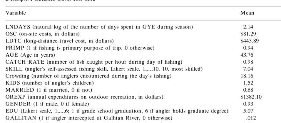
Table 1
D escriptive statistics travel cost data
S.D .
Variable M ean
LN D AYS (natural log of the number of days spent in G YE during season) 2.14 1.05
OSC (on-site costs, in dollars) $81.29 86.36
459.19 LD TC (long-distance travel cost, in dollars) $443.89
0.94
PR IM P (1 if fishing is primary purpose of trip, 0 otherwise) 0.23 43.76
AG E (Age in years) 14.43
0.98
CATCH R ATE (number of fish caught per hour during day of fishing) 1.18 SK ILL (angler’s self-assessed fishing skill, Likert scale, 1,...,10, 10, most skilled) 7.04 2.09
18.16
Crowding (number of anglers encountered during the day’s fishing) 15.72
K ID S (number of angler’s children) 1.52 1.57
0.68
M AR R IED (1 if married, 0 if not) 0.47
1555.6 $1382.10
OR EXP (annual expenditures on outdoor recreation, in dollars)
0.93
G EN D ER (1 if male, 0 if female) 0.25
5.07
ED U (Likert scale, 1,...,6; 1 if grade school graduation, 6 if angler holds graduate degree) 1.26
.012 0.32
G ALLITAN (1 if angler intercepted at G allitan R iver, 0 otherwise)
0.22
SLID E IN N (1 if angler intercepted at Slide Inn of M adison river) 0.41
0.32 0.41
YELLOWSTON E (1 if angler intercepted at Yellowstone R iver in YN P)
0.05 0.22
CABIN CR EEK (1 if angler intercepted at Cabin Creek of M adison R iver)
anglers, few (if any) good substitutes exist for these waters. Surveys were either handed to an-glers on or near the rivers or left on the wind-shields of cars at parking lots popular with anglers. In either case, a letter with an Oregon State U niversity letterhead asked anglers to com-plete and return the surveys in a pre-addressed, stamped envelope. Surveying was done at two different locations on the M adison R iver in M on-tana, known locally as Cabin Creek and Slide Inn, as well as at three different sites within YN P: Slough Creek, the G allitan R iver and the Yellow-stone R iver.
Anglers returned 386 (35%) of the surveys. Al-though this response is somewhat low, the re-sponses are much the same as those we received in personal interviews with anglers conducted in the G YE 2 years later.4 As a possible check for low
response biases, we tested if individual responses on key variables such as income and catch rate were related to returning the survey late.5 We
rejected the hypothesis that late returned re-sponses were different from non-late rere-sponses (a50.01, 2-tailed test). In addition, the propor-tions of anglers at the surveyed sites within YN P closely mimic the proportions reported by the N PS (F ranke, 1997).
The survey contained three parts. All anglers were asked to complete Part 1, which collected information on fishing quality, angler’s demo-graphic variables, travel cost and on-site costs. Part 2 was completed by anglers spending multi-ple days in the G YE, but only visiting the G YE. Part 3 was completed by multiple day anglers who were also visiting destinations outside the G YE. Part 3 collected detailed information on the other destinations visited by the angler and, from this information, we constructed the additional mileage resulting from the G YE visit.
Our sample consists of visitors arriving at the G YE by commercial plane (27%), private cars (70%), or motor homes (3%). R espondents were overwhelmingly male (93%), highly educated (the mode response for level of education was ‘gradu-ate degree’) and predomin‘gradu-ately wealthy (the mode response for income level using ten different cate-gories was ‘\$100 000’). M ost anglers viewed themselves as skilled anglers; on a scale of 1 – 10 (most skilled) the mean response was 7.04. M ost 4This latter survey was conducted by the H enry’s F ork
F oundation on the H enry’s F ork of the Snake R iver, also in the G YE.
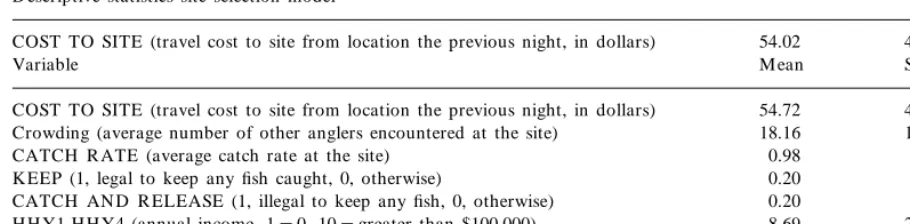
Table 2
D escriptive statistics site selection model
COST TO SITE (travel cost to site from location the previous night, in dollars) 54.02 42.02
Variable M ean S.D .
42.83 COST TO SITE (travel cost to site from location the previous night, in dollars) 54.72
Crowding (average number of other anglers encountered at the site) 18.16 15.72
CATCH R ATE (average catch rate at the site) 0.98 1.18
K EEP (1, legal to keep any fish caught, 0, otherwise) 0.20 0.40 CATCH AN D R ELEASE (1, illegal to keep any fish, 0, otherwise) 0.20 0.40 H H Y1-H H Y4 (annual income, 1=0, 10=greater than $100 000) 8.69 20.34
TYPE1-TYPE4 (1, local residence, 0, otherwise) 0.02 0.14
spent a considerable sum of money in outdoor recreation during the year (average, $1382.10). The anglers surveyed averaged slightly over 11 days fishing in the G YE during the season. The average respondent encountered slightly over 18 other anglers each day on the stream.
The data were used to estimate visitation length and site selection model. D escriptive statistics and short definitions for the variables used in estima-tion are given in Tables 1 and 2.
3.2. V isitation length
F irstly, consider the decision of how many days to visit the G YE. We separate travel costs into long-distance travel costs (LD TC) and on-site costs (OSC) (Bell and Leeworthy, 1990; H of and K ing, 1992). This formulation says that, when traveling to a distant fishery, the angler decides how many long-distance trips to make to the fishery and the number of days to spend each trip. Together, these make up the anglers’ visitation length.
The dependent variable used in modeling the number of days in the G YE is lnD AYS, the loge
of the number of days the angler spends fishing in the G YE between October and M ay. The three categories of explanatory variables are travel costs, composites of G YE site attributes including congestion and demographic variables.
3.3. V isitation length determinants
We expect that LN D AYS will be inversely re-lated to the OCS of angling. H owever, the
direc-tion of influence of LD TC is ambiguous. As LD TC increases, anglers will reduce the number of trips to the G YE, but may stay longer each trip. A substantial increase in trip duration could result in an increase in lnD AYS (Bell and Leewor-thy, 1990).
We separated LD TC from OSC differently for three different types of visitors: (1) Visitors mak-ing a smak-ingle-day trip had all costs associated with their visit allocated to on-site costs and were assigned a LD TC equal to zero; (2) Anglers mak-ing multi-day trips to the G YE, but to no other sites, were assigned OSC costs equal to the sum of their single-day travel cost to the site, the cost of the prior night’s lodging and costs for fishing equipment purchased that day; (3) Anglers visit-ing the G YE in the course of a multiple destina-tion trip were asked if their total driving distance changed due to their stop in the G YE. If individ-uals were driving through the G YE on their way to another destination and indicated that their long distance travel plans would not have changed if they had not stopped in the area, we assigned them a LD TC of zero. If their total trip length did change because of coming to the G YE, we calculated their incremental increase in mileage traveled to visit the area and added the cost of this mileage to LD TC.
1992). M otor home costs were obtained from local vendors of rental vehicles and included a base charge of $800, a rental fee of $0.16/mile for any miles over 800, as well as gasoline costs of $0.12/mile. M ileage was calculated from the R and M cN ally R oad Atlas. When there was more than one adult in the angler’s party, the calculated automobile costs were divided by the number of adults in the party.
We used survey responses to identify anglers who flew to the G YE, but we did not obtain direct information on airfare. We approximated airfares by using a sample of actual air fares from 120 U S cities to Jackson, WY and Boze-man, M T, the two most likely airports used by G YE anglers. We estimated the following equa-tion for air fares (t -statistics in parentheses):
Airfare=280.9−146.3* DUM+0.14* M L (4.14) (1.74) (4.15)
+0.07* DUM *M L (1.14)
R2
=0.81; F=76.33; N=120
where DUM=(0 or 1) depending on whether the trip was \/B1500 miles and M L is the one way mileage of the airplane trip. The vari-able DUM and its interaction with M L capture the effects of fixed costs and scale economies in the purchase of airline tickets. Predictions for airline costs were obtained by substituting mileage from the anglers’ origins into the above equation.
A measure of the opportunity cost of time was also included in LD TC, but not OSC. We calculated this cost per hour as one-third of the anglers annual income divided by an estimate of the number of hours worked per year (1920). We estimated the hours of long-distance travel as distance from the angler’s origin to the G YE divided by 50 for automobile travelers and by 300 for airline travelers.
3.4. Demographic 6ariables
D emographic variables influencing visitation length include age (AG E), a binary variable for
gender (G EN D ER ; 1, male, 0, female), marital status (1, M AR R IED ), number of children (K ID S), level of education (ED U ), annual ex-penditures for outdoor recreation OR EXP as a proxy for income (Shaw, 1991), the angler’s per-ception of her fishing skill (SK ILL). F inally, we include a binary variable, PR IM P=1 if the pri-mary purpose of the visit was fishing and 0 oth-erwise.
3.5. S ite attributes
We include two site attributes that are likely to be important in anglers’ visitation length de-cision. CATCH R ATE is the number of fish caught per h by the angler and crowding is the number of other anglers encountered by the sur-vey respondent. The myriad unmeasured at-tributes of the five surveyed sites are proxied by four dummy variables. G ALLITAN , 1 for a G allitan R iver angler and 0 otherwise; CABIN CR EEK , 1 for an angler on the M adison river near Cabin Creek; SLID E IN N , 1 for the M adison R iver near Slide Inn; and YELLOW-STON E, 1 for the Yellowstone R iver near Buf-falo F ord inside YN P. Slough Creek, a tributary of the Lamar R iver in YN P, is the referent site.
The visitation equation we estimate is
LN D AYS=b0+b1* OSC+b2 * LD TC
+b3 * PR IM P+b4* AG E
+b5 * CATCH R ATE
+b6 * SK ILL+b7 * CR OWD IN G
+b8 * K ID S+b9 * M AR
+b10 * OR EXP+b11* G EN D ER
+b12 * ED U+b13 * G ALLITAN
+b14 * CABIN CR EEK
+b15 * SLID E IN N
+b16 * YELLOWSTON E
We expect b1B0, b5\0. The signs of the
other parameters, including b2 and b7, are not
3.6. S ite selection model
We use a discrete choice, or random utility model to estimate the probability an individual visits a specific site based on a vector of congestion vari-ables at each site, c; a vector of other attributes of the sites, t and a vector of individual characteristics, x. On any given day in the G YE, the angler chooses the site that yields the highest level of utility. The mixed logit specification of the probability that an angler visits the jth site is
Prob(Si)=e(r
%c+b%t+a%x)/%(r%c+b%t+a%x) j=1, 2, ....5,
whereaand b and r are vectors of parameters to be estimated.
The 5 G YE sites are denoted: 1=G allitan R iver, 2=Slide Inn (M adison R iver), 3=Yellowstone R iver, 4=Cabin creek (M adison R iver). The refer-ent site is Slough creek. The means and S.D . of the variables used appear in Table 2.
The first discrete choice site attribute is the site-specific COST TO SITE, the cost of travel from the place the angler stayed the previous night to the site.6 We also included the average number of
anglers that our respondents encountered at each
site (crowding), the average catch rate per angling hour at the site (CATCH R ATE) and two dummy variables indicating the type of fishing regulations at the site. The first of these, K EEP=1 if it is legal to keep any of the fish caught and 0 otherwise. The second, CATCH AN D R ELEASE=1 if all caught fish must be released and 0 otherwise. The referent sites have regulations such that some types of fish may be kept and others must be released.7
M any individual characteristics were considered for inclusion in the discrete choice model. These included marital status, number of children, skill level and a dummy variable indicating if fishing was the primary purpose of the G YE visit. Based on likelihood ratio tests, two variables were retained in the estimates we report here. The first measures the respondent’s income, H H Y(J ), a ten-category scale from ‘$0’ to ‘\$100 000’, with :equal intervals. The second variable is TYPE(J )=1 if the angler resided in the local area and 0 otherwise. The (J ) suffix on H H Y and TYPE indicates that a separate coefficient is estimated for each of the four non-referent sites. Slough creek (Sj=5) is the referent site and is omitted.8
The site choice specification we estimated is
(r%c+b%t + a%x)
=r1*CR OWD IN G+b1* COST TO SITE
+b2* CATCH R ATE+b3*K EEP
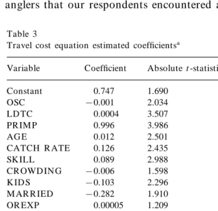
+b* CATCH AN D R ELEASE Table 3
Travel cost equation estimated coefficientsa
Absolute t -statistic
6R andall (1994) notes that the decisions such as lodging location on the previous night may be endogenous. The coeffi-cient for COST TO SITE should, therefore, be interpreted with caution.
7On Slough Creek and the Yellowstone R iver all caught fish must be released. Only on the Cabin Creek section of the M adison can fish of any species and size be kept.
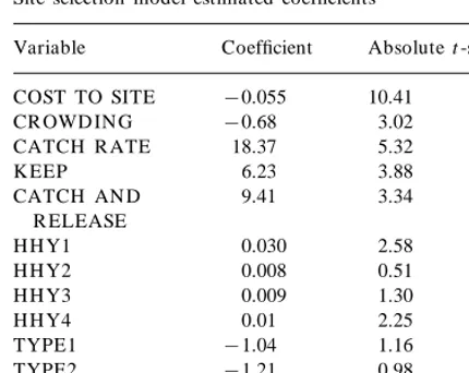
Table 4
Site selection model estimated coefficientsa
Absolute t -statistic Variable Coefficient
COST TO SITE −0.055 10.41
CR OWD IN G −0.68 3.02
Site attributes have strong influences on visita-tion length. One would expect that catching more fish is viewed positively and we find that CATCH R ATE positively influences LN D AYS. Of the lo-cation dummy variables, SLID E IN N is negative and significant. This indicates that anglers who frequent the Slide Inn area of the M adison R iver tend to spend fewer days in the G YE than those who visit Slough Creek. The estimated crowding coefficient is negative, with a t -statistic of 1.60. This provides weak evidence anglers self-regulate in response to crowding.
4.2. S ite selection estimation
The site selection model estimates are in Table 4. Overall, the estimated equation has consider-able explanatory power and most of the coeffi-cients are statistically different from zero. We reject the null hypothesis that all of the slope coefficients are zero (a50.01).
F irst consider the site attribute variables. The estimated coefficient for COST TO SITE is nega-tive as expected and statistically significant. Sites that are further away, therefore costing more to visit, are less likely to be visited by an angler who has arrived in the G YE. The estimated coefficient for crowding is negative and statistically signifi-cant (a50.01). The implication is that there is some angler self-regulation; anglers respond to increased crowding by moving to alternative sites. The large, positive and significant coefficient on CATCH R ATE indicates that anglers are very sensitive to the number of fish they catch, some even in the quality waters of the G YE. Increases in CATCH R ATE at a particular site lead to increases in the probability that a site is visited, ceterius paribus. The estimated coefficients associ-ated with K EEP and CATCH AN D R ELEASE are both positive and statistically different from zero (a50.01). Both catch-and-release manage-ment and regulations that allow any fish to be kept, encourage anglers to use a site. Complex regulations that target certain fish species or sizes for mandatory release seem to discourage visita-tion to a site. This may be due to anglers’ aver-sion to the complexities of the regulations and +a1* H H Y1+a2 * H H Y2+a3 * H H Y3
+a4* H H Y4+a5 * TYPE 1+a6 * TYPE 2
+a7* TYPE 3+a8 * TYPE 4
4. Estimation of anglers’ behavior
4.1. V isitation length estimation
The visitation length estimation results are given in Table 3. Overall, the estimated equation has substantial explanatory power and the coeffi-cients are of the expected sign. As theory predicts, OSC and LN D AYS are negatively correlated. We find LD TC and LN D AYS are positively related, as do Bell and Leeworthy (1990).
insignifi-Table 5
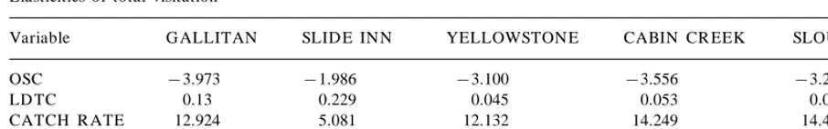
Elasticities of total visitation
YELLOWSTON E CABIN CR EEK SLOU G H CR EEK Variable G ALLITAN SLID E IN N
−3.212
OSC −3.973 −1.986 −3.100 −3.556
0.057 0.053
LD TC 0.13 0.229 0.045
14.461
CATCH R ATE 12.924 5.081 12.132 14.249
−7.079
Crowding −6.887 −4.791 −12.021 −8.286
confusion about compliance. These results suggest that the setting of harvesting regulations represents an efficacious tool available to managers to influ-ence anglers’ behavior.
Variables relating to individual characteristics add significant explanatory power to the site selec-tion model. The positive and significant coefficients for H H Y 1 and H H Y 4 indicate that, relative to the referent site (Slough Creek), higher income anglers are more likely to visit the G allitan R iver and Cabin Creek on the M adison. N one of the coefficients for TYPE 1 – TYPE 4 are individually significant, al-though they are as a group. The implication is that Slough Creek is preferred by local anglers, ceterius paribus.
4.3. Elasticities
Taking partial derivatives of the visitation and site selection equations and substituting into Eq. (1) gives own and cross elasticities of the form
[[R · Pj·(1−Pj)·zc]+Pj·[dc· R ]]·
cj T Vj
for the i=j and
[(−R · Pj· Pi)·zc]+Pj·[dc· wi· R ]] ·
ci T Vj
for i"j. The z and d refer to coefficients in the site choice visitation length equations, respec-tively, and their c subscripts refer to the associ-ated variable. F or comparison, in Table 5 we present own elasticity estimates (i=j ) for OSC9,
LD TC, CATCH R ATE and CR OWD IN G evalu-ated at the sample means.
F rom Table 5, the absolute values of the elas-ticities of CATCH R ATE are about twice those of CR OWD IN G , which in turn are twice those of OSC. A 1% increase in the CATCH R ATE (:0.1 fish per angling day) leads to a predicted 12 – 14.5% increase in visitation at four of the sites, or
:0.5 more days per season by the typical G YE angler. F or SLID E IN N the effect is only half as large. Similarly a 1% increase in CR OWD IN G (:0.20 more fellow anglers encountered in a day) leads to a 5 – 8% decrease in total visitation at four of the sites (or :0.3 days). At Yellowstone (the most crowded site) the decrease is nearly twice as large. By comparison, a 1% increase in OSC (:$0.81) would decrease total visitation by the typical G YE angler 3 – 4% (or :0.14 days) at four of the sites and by 2% at SLID E IN N .
Although CATCH R ATE and CON G ESTION may be very difficult variables for managers to affect, OSC are within their control through site-varying access fees. These fees are not currently charged for public waters in the G YE, but several privately-owned spring creeks and lakes in the G YE do have daily fees of $50 – 200. Our elasticity estimates suggest that access charges would de-crease total visitation at any given site. H owever, the results further suggest that anglers’ self-regula-tion through CR OWD IN G has about twice as strong an effect as daily access fees.
Anglers do not appear to be very responsive to increases in total trip costs, LD TC. The elasticity estimates range from 0.23 at SLID E IN N to 0.045 at YELLOWSTON E. The positive signs indicate that increases in LD TC would increase total visi-tation, but the effect would be very small. It appears that managers could charge substantially more for access to the G YE, without substan-9COST TO SITE is treated as an on-site cost for these
tively affecting visitor number or choices of sites to visit. By charging entrance fees that are invari-ant to site and visitation length, G YE managers can and do influence LD TC. This occurs in the form of weekly10 or seasonal passes now sold by
YN P. The small estimated responses are consis-tent with the recent experience of YN P managers, as noted by YN P Superintendent M ike F inley (1997). In 1995, YN P doubled its weekly and seasonal pass prices. It received few, if any, com-plaints and observed no change in visitor num-bers. This is also consistent with recent Canadian experience, where entrance fees at some parks doubled over three years, with no change in visita-tion (M cCarville et al., 1999).
There are also implications here for managers who are concerned about the incompatibility of using market methods and the pursuit of equity goals (Alden, 1997). Our results and the recent experience of YN P managers, suggest that re-source managers in the G YE can use weekly or seasonal access fees to obtain revenue, while hav-ing minimal effects on total visitation by most park users. The relatively high incomes reported by our sample of G YE anglers may also reduce any equity-based concerns that park managers have about using entrance fees for revenue purposes.
5. Conclusion
R esource managers are required to balance the wants of recreational anglers with the human impact these anglers have on the ecosystem. In the greater Yellowstone ecosystem (G YE), particu-larly in Yellowstone N ational Park (YN P), this issue is especially sensitive. M any even question whether recreational fishing is consistent with the park’s primary goals.
The empirical results presented here provide guidance in deciding which tools might be effec-tively used to guide anglers’ impacts. F irst, har-vesting regulations do influence anglers’ behavior. Anglers are encouraged to use a site by both
regulations that mandate catch-and-release for all fish and that allow any fish to be kept. They are more likely to eschew sites with complicated regu-lations that target certain fish species or sizes for mandatory release.
Secondly, anglers view crowds at fishing sites in a negative manner and self-regulate by varying their choice of fishing sites and the number of days to fish at all sites in response to the number of other anglers present. Thirdly, some types of market pricing methods are effective in influenc-ing anglers’ choices, but they need to be used with care to align methods with recreation manage-ment goals. Increases in the costs/day of fishing at a site can be effectively used to decrease the number of days that anglers visit and to shift visits from one site to others. While this effect may be consistent with the goal of managing ecosystem impacts, it may be inconsistent with equity, or other goals. Alternatively, increases in the cost per trip not related to a specific site have positive, but relatively small effects on visitation. The explanation is that increases in trip costs induce people to make fewer long distance trips; but they stay longer each trip. The net result is more visitor days. These results suggest that in-creases in the the cost of season fishing permits or park entrance fees are not likely to reduce fishing pressure, but can be used to pursue revenue goals. In contrast, charging anglers a site-specific fee for each day may be effective in managing anglers’ ecological impacts, but may be inconsistent with equity goals.
difficult to generalize to different resources. When a critical resource is threatened, managers may be more comfortable using more draconian, but pre-cise, measures such as proscription and queuing.
References
Alden, A., 1997. R ecreational users management of parks: an ecological economic framework. Ecol. Econom. 23, 225 – 236.
Bell, F ., Leeworthy, V., 1990. R ecreational demand by tourists for saltwater beach days. J. Environ. Econ. M anage. 18, 189 – 205.
Berrens, R ., Bergland, O., Adams, R ., 1993. Valuation issues in an urban recreational fishery: spring chinook salmon in Portland, Oregon. J. Leisure R es. 25, 70 – 83.
Brown, G ., M endelson, R ., 1984. The hedonic travel cost method. R . Econ. Stat. 66, 427 – 433.
Cicchetti, C., Smith, K ., 1973. Congestion, quality deteriora-tion and optimal use: wilderness recreadeteriora-tion in the Spanish peaks primitive area. Soc. Sci. R es. 2, 15 – 30.
Caulkins, P., Bishop, R ., Bowles, N ., 1986. The travel cost model for lake recreation: a comparison of two methods for incorporating site quality and substitution effects. Am. J. Ag. Econ. 68, 292 – 297.
F inley, M ., 1997. Welcome and Opening R emarks. G reater Yellowstone Coalition Conference. Bozeman, M T, U SA. F isher, A., K rutilla, J., 1972. D etermination of an optimal
capacity for resource-based recreation facilities. N at. R es. J. 12, 417 – 444.
F ranke, M ., 1997. A grand experiment. Yellowstone Sci. 5, 8 – 13.
G raefe, A.F ., K uss, F ., Vaske, J., 1990. Visitor Impact M an-agement: The Planning F ramework. N ational Parks and Conservation Association, Washington, D .C.
H of, J., K ing, D ., 1992. R ecreational demand by tourists for saltwater beach days: comment. J. Environ. Econ. M anage. 22, 281 – 291.
H unsaker, J., M arnell, L., Scharpe, F ., 1970. H ooking
mortal-ity of Yellowstone cut-throat trout. Progressive F ish-Cul-turist. 32, 231 – 235.
Jacob, G ., Schreyer, R ., 1980. Conflict in outdoor recreation: a theoretical prospective. J. Leisure R es. 12, 368 – 380. K uss, F ., G raefe, A., Vaske, J., 1990. Visitor Impact M
anage-ment: A R eview of R esearch. N ational Parks and Conser-vation Association, Washington, D C.
La Pierre, Y., 1994. Taking Stock. N ational Parks. M ay/June 35 – 40.
M cCarville, R ., Sears, D ., F urness, S., 1999. U ser and commu-nity preferences for pricing park services: a case study. J. Park. R ec. Admin. 17, 91 – 105.
M cClanahan, T., 1990. Viewpoint. Bioscience, 40, January 5. M cConnell, K ., 1988. H eterogenous preferences for
conges-tion. J. Environ. Econ. M anage. 15, 251 – 258.
N ational Park Service (N PS), 1995. R esource M anagement Plan: Yellowstone N ational Park M arch.
R andall, A., 1994. A difficulty with the travel cost methods. Land Econom. 70, 88 – 96.
Schwartz, S., 1977. N ormative Influences on Altruism. In: Berkowitz, L. (Ed.), Advances in Experimental Social Psy-chology. Academic Press, Boston, M A.
Schill, D ., G riffith, J., G resswell, R ., 1986. H ooking mortality of cutthroat trout in a catch and release segment of the Yellowstone R iver, Yellowstone N ational Park N .A. J. F isheries M anage. 6, 226 – 232.
Schneider, I., H ammitt, W., 1995. Visitor response to outdoor recreation conflict: a conceptual approach. Leisure Sci. 12, 223 – 234.
Siderelis, C., Brothers, G ., R ea, P., 1995. A boating choice model for lake valuation. J. Leisure R es. 27, 264 – 282. Shaw, R ., 1991. R ecreational demand by tourists for saltwater
beach days: comment. J. Environ. Econ. M anage. 20, 284 – 289.
Shelby, B., Vaske, J., H arris, R ., 1988. U ser standards for ecological impacts at wilderness campsites. J. Leisure R es. 20, 245 – 256.
D epartment of Transportation, U S, 1986, Costs of Owning and Operating Automobiles and Vans. Washington, D C. U .S. D epartment of Labor, 1992, CPI Annual R eport.
Wash-ington, D C.
Wilkinson, T., 1995. Crowd Contr. N at. Parks 69, 36 – 42.