SPATIOTEMPORAL PATTERNS AND ITS INSTABILITY OF LAND USE
CHANGE IN FIVE CHINESE NODE CITIES OF THE BELT AND ROAD
B. Quana,b,d,*, T. Guoc
, P. L. Liu a,b, H. G. Rend
a
College of City and Tourism, Hengyang Normal University, Hengyang 421002, People’s Republic of China; b
Hengyang Base of the International Centre for natural and cultural heritage of the UNESCO, Hengyang Normal University, Hengyang 421002, People’s Republic of China
-
([email protected], [email protected]) cSchool of Computer Science and Engineering. Hunan University of Science and Technology, Taoyuan Road, Xiangtan Hunan 411201, People’s Republic of China – [email protected]
d
School of Resource, Environment and Safety Engineering. Hunan University of Science and Technology, Taoyuan Road, Xiangtan Hunan 411201, People’s Republic of China
-
[email protected]Commission IV, WG IV/3
KEY WORDS: Urban growth, Land use change, Flow matrix, Instability, Belt and Road
ABSTRACT:
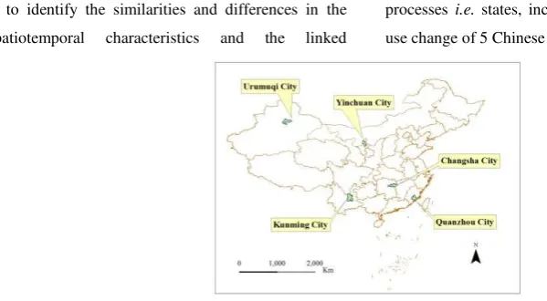
It has long recognized that there exists three different terrain belt in China, i.e. east, central, and west can have very different impacts on the land use changes. It is therefore better understand how spatiotemporal patterns linked with processes and instability of land use change are evolving in China across different regions. This paper compares trends of the similarities and differences to understand the spatiotemporal characteristics and the linked processes i.e. states, incidents and instability of land use change of 5 Chinese cities which are located in the nodes of The Silk Road in China. The results show that on the whole, the more land transfer times and the more land categories involved changes happens in Quanzhou City, one of eastern China than those in central and western China. Basically, cities in central and western China such as Changsha, Kunming and Urumuqi City become instable while eastern city like Quanzhou City turns to be stable over time.
1. INTRODUCTION
is to identify the similarities and differences in the spatiotemporal characteristics and the linked
processes i.e. states, incidents and instability of land use change of 5 Chinese cities.
Figure 1. Location map of study area in the Belt and Road of China
2. MATERIAL AND METHODS
2.1 Data sources
Remote sensing images and their resolution, data sources, data format of Quanzhou, Changsha, Yinchuan, Urumuqi, Kunming are shown in Table 1 which is in accord with the 1: 100,000 land use
classification. We consulted the land cover classification system from the China Environmental Sciences Remote Sensing Land Cover classification criteria. The land use classification system is: Built, Cropland, Orchard, Grassland, Water body, Forest, Unused land. In this study, IDRISI TerrSet and remote sensing are applied to process data.
Cities Data sources Time points
Resolution
Quanzhou I:100000 vector data in 1990 is from China
Resources and Environmental Database;
1995, 2000, 2005, 2010 Landsat TM, from the US
Geological Survey USGS;
1990 is vector;
1995, 2000, 2005, 2010
are aster;
30 m
Changsha 1990, 1995, 2000 1:100000 vector data from
China Resources and Environmental Database;
2005, 2010 the TM / ETM from the US Geological
Survey USGS;
1990, 1995, 2000 are
vector;
2005, 2010 are raster;
30m
Kunming 1990, 2000, 2008 1:100000 vector data are from
http://www.resdc.cn/Default.aspx.
2014 use Landsat 8 OL1,from geospatial data
cloud platform
1990, 2000, 2008 are
vector;
2014 is raster;
30 m
Yinchuan 1989, 1995, 2000, 2007 is the Landsat-5 TM; 2014
is Landsat-8; They are from the Chinese Academy
of International Science Data Services Platform.
1989, 1995, 2000, 2007,
2014 are raster;
30 m
Urumuqi 1989, 1999 and 2006 are the TM / ETM + remote
sensing; 2014 is TIRS; They are from Earth
System Science Data Sharing Service Platform
and the US Geological Survey USGS.
1989, 1999, 2006 and
2014 are raster.
30 m
2.2 Methods
2.2.1 Incidents and States Algorithms
In order to study the processing of urban land use changes, we applied a computer program in the language Visual Basic for Applications embedded in Microsoft Excel that interfaces with the GIS software TerrSet (Eastman 2014). A pixel’s number of Incidents is the number of times the pixel experiences a change. Incidents can range from 0, indicating complete persistence, to the number of time points
minus 1, indicating change across all time intervals. A
pixel’s number of States is the number of different
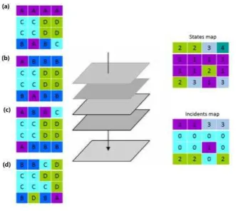
categories that the pixel represents at all time points. States can range from 1, indicating complete persistence, to the smaller of the number of time points and the number of categories (Zhang, 2011; Runfola, Pontius, 2013; Zhang , Pontius, 2016). The two algorithms measure the multi-phase remote sensing image classification in spatial in different angles. The more detail is shown in Figure 2.
Figure 2. The number of land use the Incidents and the States algorithms
Incidents and States algorithms are extracted from the changes of pixels of the different period’s remote sensing image classification results. A study area with a T-interval of remote sensing images, the results will produce T-1 transition layers and T-1 category layers, where the t-th transition layer is generated by the time interval [Yt, Yt + 1].
As shown the left part of the Figure 2 (a)-(d) represents the different periods of urban land use remote sensing interpretation data. A, B, C and D represent the different periods remote sensing interpretation categories. The right is the results of the Incidents and States algorithm. Besides, the study divides the Incidents algorithm and States algorithm into pixel-level changes in the level and pattern of changes. Pixel-level changes include changes in the number of single and multiple category changes.
For example, there are 16 pixels in
experimental data each time point. Each pixel is
marked with numbers first from left to right, then
from up to down among the 16 pixels distribution. It
is divided into two arrangements: one is based on
pixel level and another on pattern level. In the pixel
level, Incidents algorithm includes one time and many
times changes. Similarly, States algorithm includes
single and multiple category change. Taking the 1 and
2 position as example, the single category and the
multiple categories change ways in four different time
points is: A⟶A⟶A⟶B and A⟶B⟶B⟶B.
multiple incidents and states include exchange
transition and shift changes (Pontius and Santacruz,
2014). The 13 pixel position is exchange transition in
which the way is: B⟶B⟶A⟶B. While the 3, 4, 14,
16 pixel position are shift changes, which is:
A⟶B⟶A⟶C,A⟶B⟶C⟶D, A⟶A⟶B⟶D
and C⟶B⟶B⟶A.
The pattern level includes expansion and shrink
category shows expansion along with the changes of
surroundings. For example, the pixel symbolized with
5, 6 9, and 10 is C in the period of the (d). On the 11
position, it coverts D into C in the time point of (d),
which resulted in the quantity of C being increased. In
contrast, the shrink mode refers to the specific land
category shows decreased along with the changes of
surroundings.
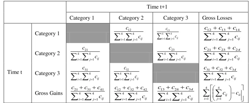
2.2.2 Based on Flow Matrix of urban land use
change instability provides a simple theoretical basis for the comparison
of the transfer and linking patterns to processes. information, is a method of measuring urban land use change and it is different from the transition matrix. The transfer matrix shows the size conversions. The Flow Matrix represents the total size of the amount transferred from class i to class j.
Time t+1
Category 1 Category 2 Category 3 Gross Losses
Time t
Table 2. The Flow Matrix form (Runfola, Pontius, 2013)
(2) Based on Flow Matrix to calculate urban land use change instability
Eq. 1 and Eq. 2 are the foundation of calculating urban land use instability. Eq.1 changes calculated observe intensity S in each time interval; the Eq.2 calculated uniform intensity U of the entire study period. After calculating the observe intensity in each time interval, we compared with uniform intensity which is compares S to U. if S > U, then the change is relatively fast for that time interval. If S <U, then the change is relatively slow for that time interval. (Aldwaik, Pontius, 2012; Pontius, Gao et al., 2013;
Zara, João, Pontius, 2016; Enaruvbe, Pontius, 2015).
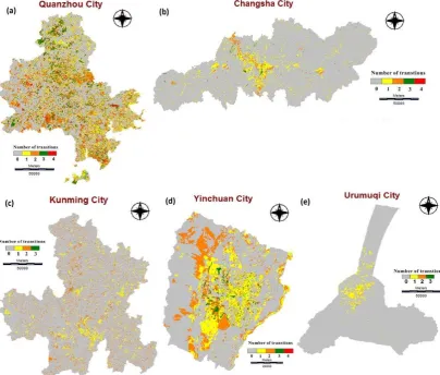
legend colors indicate more frequent transitions overtime. In these figures, zero in the legend indicates persistence across the time extent. The maximum value for any pixel in these maps is equal to the number of time intervals.
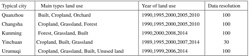
Typical city Main types land use Year of land use Data resolution
Quanzhou Built, Cropland, Orchard 1990,1995,2000,2005,2010 100 Changsha Cropland, Grassland, Forest 1990,1995,2000,2005,2010 100
Kunming Forest, Grassland, Built 1990,2000,2008,2014 100
Yinchuan Cropland, Built, Grassland 1989,1995,2000,2007,2014 30 Urumuqi Cropland, Grassland, Built, Unused land 1990,1999,2006,2014 100
Tab. 3 The characteristics of typical city land use data
Figure 3. The Incidents map in the typical cities.
Figure 3(b) is a four interpretation of remote sensing data obtained the transition frequency of Urumuqi urban land use. The 1 time land category transition is mainly accounted for the 91%. Generally, Cropland, Grassland and Bare were converted to the Built, which happens mainly in the Midong and Tianshan District. The 2 times only accounted for 8.6% whose land conversion is as follows: Grassland
→ Cropland →Built. Figure 3 (c)-(e) shows the times of transition for Kunming City. In Kunming, the 1 and 2 times of land transition are accounted for 34.7% and 64.8%, respectively. In the northwest of Luquan Yi and Miao Autonomous County and Dongchuan District are mainly forest, Cropland and Grassland. Panlong, Wuhua Guandu District is mainly construction land. It appears around the Xishan, Jinning, Chenggong District are water in the form of the distribution network. The 1 time and 2 times transfer are mainly for Cropland, Forest and Grassland
carrying changes between both or all three. In the Jinfeng District, Xingqing district and eastern Helan County there is distribution of Built and Crop land. In Xixia, Yongning County, and western Helan County are distribution of forest, grassland and unused land. Yinchuan City distributed waters in the east. The land that transfer 1 time and 2 times are mainly Cropland, Forest and grassland. For Yinchuan City, land that transfer 1 and 2 times are mainly distributed in the Jinfeng District, Xingqing district, northern Xixia district and central Helan Mountain. The occurrence
of urban land use change is: Cropland →Built, Forest
→ Built and Unused land → Cropland, and so on. For Changsha, the land that transfers 1 and 2 times accounted for 75.6% and 20.2%, which happens in Liuyang River and Changsha urban area.
accounting for 97.8% and 91%, respectively. Land use change happened in the two areas mainly in a way of exchange. Quanzhou occurs one, two and three times with the way of swap changes, accounting for 31.2%, 43.4% and 18.5%, respectively. Changsha and Yinchuan were mainly in 1st and 2nd times change. In short, we can conclude that the 1 time transfer happened in five cities mainly is Cropland being
converted to Built. And on the whole, the more times of land transfer in the developed eastern coastal region of China, e.g., Quanzhou City is more than that of central and western region. The reason possibly is that the land change tend to drag on growth in developed eastern coastal region of China. In this case Quanzhou pays attention to the forest cultivation and protection.
Figure 4. The land use change of Incidents
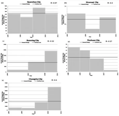
We calculate the observed changes S and uniform intensity based on Eq. 1 and Eq. 2 in Figure 5. We can see that except the Yinchuan City, the cities in central and western China such as Changsha, Kunming and Urumuqi City become instable while eastern city like Quanzhou City turns to stable over time. Obviously, from the instability perspective, the
cities of central and western China are in the opposite direction to the cities of eastern China. It shows interesting patterns that some cities such as Changsha and Kunming are accelerating land change while Quanzhou is decelerating or regulating the speed of land change.
Figure 5. Land use instability: (a) The most stable cities, (b) The mid-ranked instability, (c) - e The most
Figure 6 shows that regional comparison in typical urban change instability. If it is above the Uniform line, it belongs to unstable. And more far distance from the Uniform line of instability, more unstable land use change is. Quanzhou and Urumuqi’s R value is below the Uniform line of instability, indicating that it is stable in land use change. And Quanzhou is more stable than Urumuqi. While Changsha City is the most the unstable among the five
cities. In the five cities, the instability of urban land use change from small to large is as follows: Quanzhou, Urumuqi, Yinchuan, Kunming, Changsha City. The reason possibly is that the cities in the central and western China are experiencing earlier and middle urbanization stage while eastern city such as Quanzhou City has already entered into the later stage of urbanization.
Figure. 6 Comparison of the land use change with instability in typical cities.
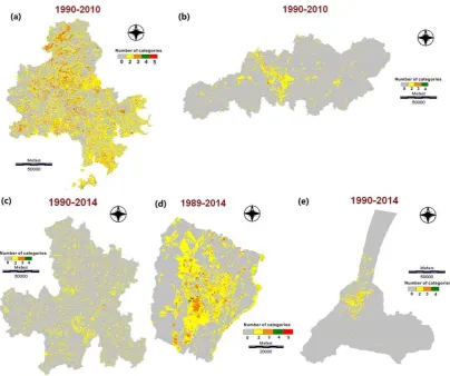
3.2 States maps in land use change
Figure 7. is the categories transfer of 5 typical cities in land use change. Figure 7 (a) shows there are 5 land categories changed in Quanzhou among the six time intervals. The change happens mainly among 2 or 3 categories, i.e., Unused land →Built, Forest → Orchard → Built. And it occurs mainly in Dehua, Yongchun County and Jinjiang City. The changes between 2 categories and 3 categories are accounted for 75% and 23.4%, respectively. In the Figure 7 (b), it occurs in around central lower-lying basin close to the Xiangjiang River riparian zone. Specifically, it mainly concentrated in the urban area of Changsha City and Wangcheng County where Cropland and Forest were converted to Built. From the Figure. 7 (c), we can see that There are 4 categories transition at most in Kunming but the change most is among the 3 categories. It is mainly located in the northern Dianchi Lake, i.e., Xishan, Wuhua and Guandu District. The change was adopted in this way: Forest→ Crop
Figure. 7 The States map in the typical cities.
Figure.8 compares the regional differences and commonalities of land use change states among the five typical cities. Quanzhou, Changsha, Yinchuan and Urumuqi mainly had the transfers between 2 categories, which accounts for their 75%, 96%, 85.9% and 95.4%, respectively. Also, Kunming and Quanzhou Cities have a longer bar than the other cities in the “3 to 5 categories transfers”. But
Kunming changes mainly depends on shift which is the component of allocation difference(Pontius et al. 2014).The reason is that terrain and climate in Kunming have an impact on this transition. From the view of regional difference in China, except the Kunming the eastern region, i.e., Quanzhou City has more land categories involved changes than those cities in central and western region, i.e. Changsha, Yinchuan and Urumuqi City.
4. CONCLUSIONS
This article used Flow Matrix, Incidents and States
algorithms to analyze land use change instability in
five node cities of China in the belt of Silk Road. On
the whole, the more land transfer times and the more
land categories involved changes occurs in Quanzhou
City of eastern China than that in central and western
China. Basically, the cities in central and western
China such as Changsha, Kunming and Urumuqi City
become instable while eastern city like Quanzhou City
turns to be stable over time.
ACKNOWLEDGEMENTS
Key Project of Hunan Provincial Department of Education of China and the National Natural Science Foundation of Chinafunded this work via grant 17A067 and grant 41271167. Also Recruitment Program of High-end Foreign Experts of the State Administration of Foreign Experts Affairs of China funded this work via grant GWD201543000243. The authors thank Robert Gilmore Pontius Jr, from Clark University, USA who gave us the programming on the Incidents algorithm and States algorithm.
REFERENCES
Aldwaik S., Pontius Jr R G., 2013. Map errors that could account for deviations from a uniform intensity of land change. International Journal of Geographical Information Science, 27(9), pp. 1717-1739.
Aldwaik S., Pontius Jr R G., 2012. Intensity Analysis to unify measurements of size and stationarity of land changes by interval, category, and transition. Landscape and Urban Planning, 106, pp. 103-114.
Aldwaik S., 2012. Fundamental concepts of intensity analysis to understand changes among categories. USA, Clark University, pp. 125-137.
Costanza R., R. d'Arge., 1997. The value of the world's ecosystem services and natural capital. Nature, 387(6630), pp. 253-260.
Chi W F., Shi W J., Kuang W H., 2015. Spatio-temporal characteristics of intra-urban land cover in the cities of China and USA from 1978 to land-use dynamics in a fast developing city using the modified logistic cellular automaton with a patch-based simulation strategy. International Journal of Geographical Information Science, 28(2), pp. 234-255.
Chneider A S., Mertes C M., Tatem A J., 2015. A new urban landscape in East–Southeast Asia, 2000–2010. Research Letters, 10, pp. 1-14.
Chen G L., Yang W M., Chi W F., 2013. Analysis of land use time-space Change characteristic in Kunming city. Anhui Agricultual Science Bulletin, 19(22), pp.10-13.
Chen Y L., Xin B G., LI X Q., 2015. The Preliminary Research on Relationship between the Change of Land Use and Urbanization in Changsha from 2003 to 2013. Economic Geography, 35(1), pp. 149-154.
Chen M., Liu W., Tao X., 2013. Evolution and
Eastman J R., 2014. TerrSet Geospatial Monitoring and Modeling System. Worcester, MA: Clark University, pp. 345-389.
Gu C L., Wu L Y., Cook I., 2012. Progress in research on Chinese urbanization. Frontiers of Architectural Research, 1, pp. 101–149.
Holden E., 2004. Ecological footprints and sustainable urban form. Journal of Housing and the Built Environment, 19(1), pp. 91-109.
Huang J C., Chen S Q., 2015. Classification of China´s urban agglomerations. Progress in Geography, 34(3), pp. 290-301.
Huang Z J., Wei D., He C F., 2015. Urban land expansion under economic transition in China: A multilevel modeling analysis. Habitat International, 47, pp. 69-82.
Huang Y., Li F., Bai X., et al, 2012. Comparing vulnerability of coastal communities to land use change: analytical framework and a case study in China. Environmental Science & Policy, 23, pp. 133-143.
Kuang W H., Chi W F., Shi J., 2014. The spatial and temporal differences of urban interior land cover structure in China and the United States metropolitan area. Acta Geographica Sinica, 69(7), pp. 883-895.
Gu C L., Pang H F., 2008. Study on spatial relations of Chinese urban system: Gravity model approach. Geographical Research, 27(1), pp. 1-12.
Lambin E F., Geist H J., Agbola S B., 2001. The cause of land-use and land-cover change: moving beyond the myths. Global Environmental Change, 11, pp. 261-269.
Lei S., 2014. Comparison of Land Use Changes between Case Areas from the Developed East and Less Developed Central China: A Case Study of the Changsha and Quanzhou City. Hunan: Hunan University of Science and Technology, pp. 23-30.
Liu J Y., Zhang Q., Hu Y F., 2012. Regional
Differences of China’s Urban Expansion from Late
20th to Early 21st Century Based on Remote Sensing Information. Chinese Geographical Science, 22 (1), pp. 1–14.
Liu R., Zhu D L., 2010. Methods for Detecting Land Use Changes Based on the Land Use Transition Matrix. Resources Science, 32(8), pp. 1544-1550.
Karacsonyi D., Chang K., 2014. Comparison of urban land expansion and population growth in the Taipei metropolitan region. Global Environmental Research, 18: (2), pp. 183-190.
Pontius Jr R G., Gao Y., Giner N M., 2013. Design and interpretation of Intensity Analysis illustrated by land change in Central Kalimantan, Indonesia. Land, 2(3), pp. 351-369.
Pontius Jr R G., Alí S., 2014. Quantity, Exchange, and Shift Components of Difference in a Square Contingency Table. International Journal of Remote Sensing, 35 (21), pp. 7543–54.
Qiao W F., Sheng Y H., Wan B., 2013. Land use change information mining in highly urbanized area based on transfer matrix: A case study of Suzhou, Jiangsu Province. GEOGRAPHICAL RESEARCH, 32(8), pp. 1497-1507.
Quan B., Bai Y., Romkens M J M., et al, 2015. Urban land expansion in Quanzhou City, China, 1995-2010. Habitat International, 48, pp.131-139. Matrix. International Journal of Geographical Information Science, 27(9), pp. 1696-1716.
Schneider A., Mertes C M., 2014. Expansion and growth in Chinese cities, 1978–2010. Environmental Research Letters, 9, pp. 024008.
Liu J., Dietz T., et a, 2007. Complexity of coupled human and natural systems. Science, 317 (5844), pp. 1513-1516.
Wu J S., Liu H., Peng J., 2014. Hierarchical structure and spatial pattern of China's urban system: Evidence from DMSP/OLS nightlight data. Acta Geographica Sinca,69(6), pp. 759-770.
Xiao Z K., 2012. Urban Land Use and Land Cover Change and its Driving Factors: A case study of the Changsha-Zhuzhou-Xiangtan. Xiangtan: Hunan University of Science and Technology, 2012, pp. 45-51.
Yao Y L., 2014. Spatiotemporal Variation Characteristics and Causes of Land Surface Temperature in Typical City of Northwest Oasis. Gansu: Northwest Normal University, 2014, pp. 54-62.
Zara T., João C M., Pontius Jr R G., 2016. Evidence for deviations from uniform changes in a Portuguese Water bodyhed illustrated by CORINE maps: An Intensity Analysis approach. Ecological Indicators, 66, pp. 382–390.
Zhang Z X., Zhao X L., Wang X., 2012. Monitoring land use in China by remote sening. Beijing, China: Star Map Press, pp. 231-238.
Zhang Y J., Pontius R G., 2016. Method to summarize change among land categories across sequential time interval. Cartography and Geographic Information Science, In press.