DETECTION OF DISEASE SYMPTOMS ON HYPERSPECTRAL 3D PLANT MODELS
Ribana Roschera†∗
, Jan Behmanna†
, Anne-Katrin Mahleinc, Jan Dupuisa, Heiner Kuhlmanna, Lutz Pl¨umera
a
University of Bonn, Institute of Geodesy and Geoinformation, Bonn, Germany -(ribana.roscher, jbehmann, j.dupuis, heiner.kuhlmann, pluemer)@uni-bonn.de c
University of Bonn, Institute of Crop Science and Resource Conservation - Phytomedicine, Bonn, Germany - [email protected]
Commission VII, WG VII/4
KEY WORDS:Hyperspectral 3D plant models, close range, anomaly detection, sparse representation, topographic dictionaries
ABSTRACT:
We analyze the benefit of combining hyperspectral images information with 3D geometry information for the detection ofCercospora
leaf spot disease symptoms on sugar beet plants. Besides commonly used one-class Support Vector Machines, we utilize an unsu-pervised sparse representation-based approach with group sparsity prior. Geometry information is incorporated by representing each sample of interest with an inclination-sorted dictionary, which can be seen as an 1D topographic dictionary. We compare this approach with a sparse representation based approach without geometry information and One-Class Support Vector Machines. One-Class Sup-port Vector Machines are applied to hyperspectral data without geometry information as well as to hyperspectral images with additional pixelwise inclination information. Our results show a gain in accuracy when using geometry information beside spectral information regardless of the used approach. However, both methods have different demands on the data when applied to new test data sets. One-Class Support Vector Machines require full inclination information on test and training data whereas the topographic dictionary approach only need spectral information for reconstruction of test data once the dictionary is build by spectra with inclination.
1. INTRODUCTION
Hyperspectral images are an important tool for assessing the vi-tality and stress response of plants (Fiorani et al., 2012; Mahlein et al., 2012; Behmann et al., 2014). In recent time, sensor tech-nology for hyperspectral plant phenotyping has significantly im-proved in resolution, accuracy, and measurement time and is in-tegrated into commercial phenotyping platforms.
The identification of disease symptoms using hyperspectral im-ages is an established approach. Due to the unknown statis-tical distributions of hyperspectral data and disease symptoms, methods from the machine learning domain are used frequently. Applications cover direct classification of spectra (Moshou et al., 2004), combined analysis of multiple vegetation indices (Behmann et al., 2014) and derivation of new, disease specific indices (Mahlein et al., 2013). Supervised approaches like neural networks (Wu et al., 2008), Support Vector Machines (Rumpf et al., 2010) and LDA (Suzuki et al., 2008) and unsupervised ap-proaches like Self-Organizing Maps (SOM; Moshou et al., 2002) are used. Since label information for disease symptoms are hard to obtain and oftentimes erroneous, one-class classifiers (e.g. , Sch¨olkopf et al., 2001; Tax and Duin, 2004) and unsupervised approaches are promising (e.g. , Wahabzada et al., 2015).
Simultaneously with the improvement of hyperspectral sensors, sensor technology for the assessment of 3D geometry is consid-erably improving. A common application for analyzing 3D point clouds of plants is the segmentation of a plant into different or-gans like leaves, stems and fruits like berries (Paulus et al., 2013b; Roscher et al., 2014).
Combining both data types, hyperspectral images and 3D point clouds, to a hyperspectral 3D plant model is the recent step
∗
Corresponding author
†R. Roscher and J. Behmann contributed equally to this work
(Behmann et al., 2015a). Based on the complementary charac-teristics of both information layers several application using the synergy of spectral and spatial features are possible.
Hyperspectral 3D plant models can be generated in multiple ways. Liang et al. (2013) have generated hyperspectral 3D mod-els by observing a plant from multiple viewpoints with a full frame hyperspectral camera. These perspective images are com-bined to a 3D model by detectors for homologous points and the structure from motion principle. A similar approach was applied to crop surfaces using a unmanned aerial vehicle and a full frame hyperspectral camera that captures all bands simultaneously by (Bareth et al., 2015). The resulting crop surface models allow to extract plotwise height information and to integrate these into the spectral analysis. The combination of separately sensed spectral and spatial information was applied to solid objects in the context of compressed sensing by (Kim et al., 2011). They combine a 3D triangulation sensor with a multi-spectral camera and a rotating table to generate spectral 3D models of solid objects.
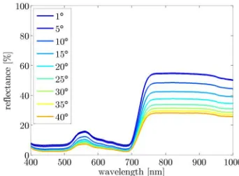
Figure 1: Average hyperspectral plant signatures for specific in-clination angles.
show-samples (e.g. , Soltani-Farani et al., 2013; Chen et al., 2011) or learned from them (e.g. , Yang et al., 2014; Charles et al., 2011). More sophisticated approaches use structured sparsity in order to integrate prior knowledge such as homogeneity assumptions into the solution (Bach et al., 2012). In this way, actual structure in the data can be modeled rather than unimportant effects from specific samples leading to overfitted solutions.
Sparse representation has also been used for outlier/anomaly de-tection by e.g. Adler et al. (2013). In this work an extra error term is introduced into the optimization function to account for all anomalies which cannot be explained well by a weighted lin-ear combination of dictionary elements. Thus, this approach is based on same assumption as one-class classifiers. We use a sim-ilar strategy based on this assumption in our paper by using a topographic dictionary in order to combine spectral as well as prior information about the geometry of the plant. Topographic dictionaries are dictionaries in which neighboring dictionary ele-ments show similar weights to input signals (Kavukcuoglu et al., 2009; Mairal et al., 2011). Their usage can promote rotation- and translation-invariant features, which is especially useful for ro-bust object recognition. Generally, the dictionary is learned from data to be topographic and develops a typical structure. In our work, the learning step is omitted, since we exploit the inclina-tion informainclina-tion to construct a sorted dicinclina-tionary, which can be seen as an 1D topographic dictionary. Fig. 1 shows some of the used dictionary elements with their respective inclination derived from 3D information of the plant. As can be seen the signal show a typical behaviour depending on the inclination.
The present paper is - to our knowledge - thefirst study that com-bines plant geometry and spectral information for detecting dis-ease symptoms in the close range. We apply our framework on sugar beet plants which are partially infested byCercosporaleaf spot disease. We employ prior knowledge about geometry and spectral characteristics to build a topographic dictionary, which is used within a sparse representation framework with group spar-sity. Furthermore, we apply feature stacking within One-Class Support Vector Machines (OCSVM; (Tax and Duin, 2004)) to integrate the geometry to show its positive effect. This allows a comparison of these different integration approaches and analysis methods.
This paper is structured as follows: Sec. 2. describes the used plant material, sensors and the combination of their geometry and spectral information. Sec. 3.1 introduces sparse represen-tation and its usage in our framework. OCSVM are introduced and the application of these methods for disease detection is out-lined in Sec. 3.1.2. In our experiments (Sec. 4.) we analyse dif-ferent aspects for the detection ofCercosporadisease symptoms and compare sparse representation with topographic and standard dictionary to OCSVM.
2. DATA
2.1 Biological material
The applications for hyperspectral 3D plant models are demon-strated by a preliminary study with sugar beet plants partially
in-phenotyping. For the experiments, plants, cv. Pauletta (KWS, Einbeck, Germany) were cultivated for 8 weeks in a controlled environment in a greenhouse. To demonstrate the ability of hy-perspectral 3D plant models for a detailed and improved disease detection, plants were inoculated withCercospora beticola, the causal agent ofCercosporaleaf spot. Three plants, one healthy and two infected, were observed by the sensor systems and hy-perspectral 3D plant models were generated based on these mea-surements.
2.2 Sensors
Hyperspectral cameras record the reflected radiation at narrow wavelength bands with a high spatial resolution in a definedfield of view. The hyperspectral pushbroom sensor unit used in this study was the VISNIR-camera ImSpector V10E with 1600 pixel observing a spectral signature from 400 to 1000 nm (Specim, Oulu, Finland) in nadir position. Its viewing plane is moved lin-early across the plant. The measured images are radiometrically normalized by subtracting the dark frame and by calculating the ratio to a white reference panel. The assessment of plant shapes requires 3D imaging techniques that handle the non-regular sur-face and the non-solid characteristics of the plant architecture. In this study, a Perceptron laser triangulation scanner (Perceptron Scan Works V5, Perceptron Inc., Plymouth MI, USA) is used. By coupling with a measuring arm (Romer Infinite 2.0 in 2.8m version) it provides an occlusion-free option for close-up imag-ing of plants with a point reproducibility better than 0.1 mm. It is chosen due to its high resolution and accuracy and has been successfully applied for 3D imaging of various plants (Wagner et al., 2011; Paulus et al., 2013a).
2.3 Combination of hyperspectral image and geometry
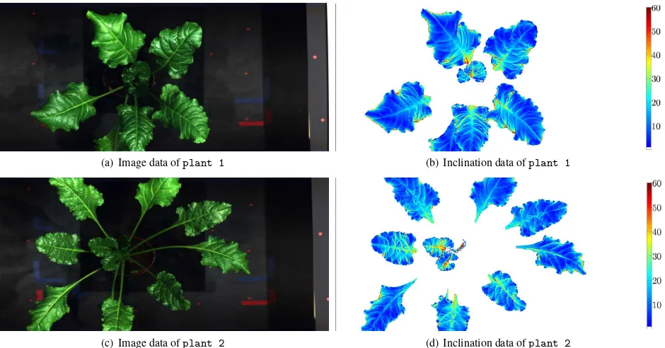
(a) Image data ofplant 1 (b) Inclination data ofplant 1
(c) Image data ofplant 2 (d) Inclination data ofplant 2
Figure 2: RGB image of both data setsplant 1andplant 2and their respective inclination information in degree.
3. DETECTION FRAMEWORK
3.1 Methods for Anomaly Detection
As label information are erroneous and its generation is related to great effort, the application of one-class classifiers and unsuper-vised approaches is favorable for stress detection on plants. We use four different approaches for detection of disease symptoms comprising sparse representation with topographic and standard dictionary and OCSVM with and without stacked inclination fea-ture. For all approaches we only provide negative examples by using an image of a healthy plant without desease symptoms. Treating these healthy samples as normal allows to characterize the anomaly of disease symptoms in the remaining images. In the following the two methods are explained in more detail and approach for the detection of disease symptoms is introduced.
3.1.1 Sparse Representation with Topographic Dictionaries
In terms of basic sparse coding a(V ×1)-dimensional test sam-plexcan be represented by a weighted linear combination of a few elements taken from a(V ×N)-dimensional dictionaryD, so thatx=Dα+ǫwithǫbeing the reconstruction error. The
parameter vector comprising the weights is given byα.
Assuming the dictionary elements were constructed using geom-etry as well as spectral information, the whole dictionary is sorted regarding the inclination. The dictionary is divided into overlap-ping groupsGi, i = 1, . . . , I, where one group comprises the indices of neighboring dictionary elements. The sparsity groups should not be confused with inclination groups, since one sparsity group can contain multiple inclination groups. The optimization functionLwith group sparsity is given by
L=||Dα−x||+λ
i
j∈Gi
wjα2
j (1)
The weights αare smoothed with Gaussian filter weights w, where the width of the kernel is chosen to by around1/3of the number of group elements. Since the groups are overlapping, the weightsαwill vary smoothly over neighboring groups. We use
group orthogonal matching pursuit as an approximation to solve for the minimization in (1) using the approach presented in Szlam et al. (2012). The maximum number of dictionary elements is re-stricted toW.
V×I V ×N
N×I
x
=
D α
. . . . . .
. . . . . .
. . . . . . ..
. ..
. ... ... ..
. ...
Figure 3: Schematic illustration of sparse representation. Differ-ent inclination groups in the dictionary are illustrated in differDiffer-ent colors, whereas sparsity groups may contain multiple inclination groups. Color intensity indicate the value of the weight.
3.1.2 One-class Support Vector Machines As second
ap-proach we use OCSVM Tax and Duin (2004), an established anomaly detector. The used OCSVM classifier derives a spheri-cal decision boundary separating a given sample set from the re-maining feature space. As this decision boundary represents the sample sets and provides a specific type of distribution model, the used method is called Support Vector Data Description (SVDD). Compared to density estimation methods, OCSVM deal well with sparsity of high dimensional data, which generelly leads to the curse of dimensionality.
3.2 Detection of Diseases
Both presented approaches yield different outcomes which can be utilized for the detection of disease symptoms (Tab. 1). For OCSVM the distance to the hyperplane is used as single output to be analyzed. For sparse representation the following outcomes can be qualified for analysis:
lies with similar spectral characteristics to be reconstructed by similar dictionary elements, since these pixels mostly have the same nearest neighbor in feature space. As a post-processing step for this outcome, we utilize morphological operators to improve the spatial analysis of dominant dictio-nary elements, e.g. by removing too small regions with the same dominant dictionary element.
The outcomes can also be combined by e.g. multiplication.
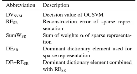
Abbreviation Description
DVSVM Decision value of OCSVM
RESR Reconstruction error of sparse repre-sentation
SumWSR Sum of weightsαof sparse
representa-tion
DESR Dominant dictionary element used for sparse representation
DE+RESR Dominant dictionary element combined with RESR
Table 1: Abbreviations for the outcomes of the used disease de-tection methods
The different outcomes are used to detect the center points of dis-ease symptoms by the following workflow: First, the background is automatically removed as 3D information is not available there. Furthermore, we removed the leaf borders from the evaluation by eroding the binary image of available inclination by10px. At last, we perform a peak detection with non-maxima suppression for each pixel in the image (c.f. Section 4.1.3) . Since disease symptoms of the plant can lie close to each other, the threshold for the non-maxima suppression has to be chosen regarding im-age resolution and prior information about the illness.
4. EXPERIMENTS
4.1 Experimental Setup
4.1.1 General Setup In our experiments we analyze two
im-ages (see Fig. 2) of plants with given data as described in Section 2.. One healthy plant with inclination information is used to build the dictionary. For construction of the dictionary we randomly se-lect 10 samples per inclination group, where on group is defined by all samples with the same inclination after rounding. Samples are discarded, which are too dissimilar regarding the standard de-viation to the average in one inclination group. Generally, these are samples from leaf veins, specular reflections and other out-liers. The detection of disease symptoms is performed using the criteria mentioned in Sec. 3.2, where several outcomes are com-bined by multiplication. Since using the dictionary elements as training data for OCSVM turned out to result in low accuracies, we randomly choose 20 samples per inclination group. The train-ing set need to include samples from leaf veins and specular re-flections to ensure high accuracies. Before applying OCSVM, the data set is Z-normalised, i.e. each feature is normalized to have
sparsity group size of|G|= 16with an overlap of14. We applied OCSVM in two different setups, once without using inclination and once with pixel-wise inclination as additional and weighted stacked feature. The idea behind this feature stacking approach is to define an anomaly in the geometric context when compared to other spectra with similar inclination. The crucial factor in apply-ing OCSVM is the specification of optimal values for the hyper-parametersν(cost on number of support vectors) andγ(kernel width). In the absence of labeled training data of two classes, we specify an outlier rate of 1% as expected leading to reasonable re-sults. Using the SVDD implementation in LIBSVM 3.18 (Chang and Lin, 2011), we optimized the two parameters using cross val-idation with a grid optimization leading to the parameter values C= 1andγ= 1.2·10−4
for the spectral data set andC= 0.46 andγ = 6.1·10−5
for the data set that utilizes also inclination. The feature weightw = 0.3is used for the inclination, which leads to visually optimal results.
4.1.3 Evaluation Criteria Due to the error-prone labeling of
the exact area of the symptoms, we decided to exclude this effect from the analysis by relying only on the symptom centers which are labeled more robust. Therefore, the detected symptom centers and the corresponding strengths of the prediction are the analysis output and the base for the result evaluation.
In order to evaluate our proposed framework, we use precision-recall curves and receiver operating characteristics (ROC). For this, the true positives rate (tp), false positives rate (fp) and false negatives rate (fn) is computed to derive precision, which is de-fined astp+fptp , and recall, which is defined astp + fntp . As evaluation measure we compute the area under curve (AUC). The higher the value the better performing the algorithm.
4.2 Results and Discussion
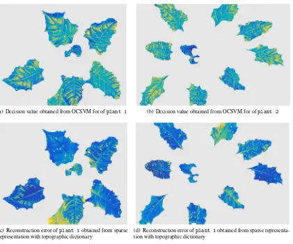
In our experiments we could observe that all outcomes presented in Sec. 3.2 could serve as indicator for disease symptoms. Fig. 4 shows the reconstruction error of the sparse representation-based approach with topographic dictionary and the decision value ob-tained by OCSVM. Both outcomes may serve as indicator for a detection of disease symptoms. As expected, the reconstruction error of the sparse representation approach as well as the deci-sion value obtained by OCSVM is higher for pixel with disease symptoms than for healthy pixels. While OCSVM show a high variability within each leaf and only small differences between leafs, the sparse representation approach shows a small variabil-ity within a leaf but large differences between leafs. Fig. 5 show a larger part of each test image for sparse representation with to-pographic and standard dictionary. Both approaches show the similar weakness to detect leaf veins as potential anomaly, how-ever they are more visually robust to specular reflections than OCSVM.
(a) Decision value obtained from OCSVM for ofplant 1 (b) Decision value obtained from OCSVM for ofplant 2
(c) Reconstruction error ofplant 1obtained from sparse representation with topographic dictionary
(d) Reconstruction error ofplant 1obtained from sparse representa-tion with topographic dicrepresenta-tionary
Figure 4: Indicator of disease symptoms obtained by sparse representation with topographic dictionary and OCSVM with inclination information. Blue color indicate a low value and yellow colors a high value.
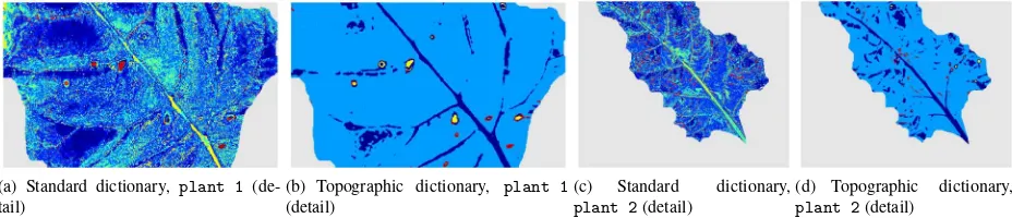
Also, leaf veins are reconstructed by mostly one, dominant dic-tionary element, however, in most cases a different one compared to pixel with diseased symptoms. Thus, using the dictionary ele-ment as indicator for diseases, leaf veins and potential areas with disease symptoms can be distinguished from each other. This is advantageous over using the reconstruction error or the sum of the weights, which show a similar behavior for disease symp-toms and leaf veins. However, the identification of the dominant element can be challenging, e.g. as soon as single, round disease areas conflate to larger areas. We could further observe that the usage of a topographic dictionary result in smoother results, so that grouping of dominant dictionary elements yield more reli-able regions (see Fig. 6). A descrease of the group size results in more used dominant dictionary elements.
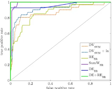
Fig. 7 as well as Tab. 2 show quantitative results. The sparse rep-resentation approach reached in most cases better results when compared to OCSVM. Detection of disease symptoms with re-construction error only results in most cases in the lowest accu-racies, because false negatives arising from leaf veins or other anomalies cause a loss in accuracy. Although the sum of the weights tend to be higher for pixels with disease symptoms, also this criteria yield worse results especially for topographic dic-tionaries and thus, is not distinctive enough for the detection of the symptoms. Although the usage of the dominant dictionary elements sometimes achieve the highest accuracy of100%, this result must be critically examined because this criterium tend to underestimate diseases. I.e. , all detected disease symptoms are correct, but only about 3/4 of all disease symptoms were de-tected. In most cases the usage of a topographic dictionary lead to a gain in accuracy. The reason for this is, as indicated earlier,
the outcomes are smoother when using a topographic dictionary and thus, the results are less effected by noise.
OCSVM achieves in both configurations and on both data sets a competitive detection accuracy of Cercospora symptoms as anomalies, however, OCSVM need more training than sparse representation-approach to achieve good results. As sparse rep-resentation, OCSVM without inclination information sometimes fail in separating leaf regions with specular reflections from the disease symptoms. Therefore the precision of the OCSVM with-out inclination is reduced. An interfering problem was the er-roneously detection of leaf veins as symptoms. As this is not related to a specific inclination it cannot be compensated by the additional inclination information. As counter measure, the train-ing set from the healthy plant should be sampled in a way that samples of leaf veins are included sufficiently.
Figure 5: Detailed illustration of reconstruction error obtained by sparse representation with topographic and standard dictionary (i.e. , no group sparsity). Blue color indicate a low value and yellow colors a high value.
(a) Standard dictionary, plant 1 (de-tail)
(b) Topographic dictionary, plant 1 (detail)
(c) Standard dictionary, plant 2(detail)
(d) Topographic dictionary, plant 2(detail)
Figure 6: Color coded indices of dominant dictionary elements for sparse representation with topographic and standard dictionary (i.e. , no group sparsity).
also improve the result quality.
5. CONCLUSION
We could show the benefit of combining hyperspectral informa-tion and geometry in terms of inclinainforma-tion angles for the detecinforma-tion of disease symptoms on plants. Our experiments confirmed for One-Class Support Vector Machines as well as a sparse represen-tation based approach with group sparsity prior a gain in accu-racy when incorporating geometry information in terms of incli-nation. However, the sparse representation-based approach only needs inclination information for building the dictionary and not for spectral reconstruction of the plant image of interest, whereas One-Class Support Vector Machines also need inclination infor-mation for training and classification to achieve a good result.
As it become visible in our experiments, the investigated anomaly detection methods have different strengths. OCSVM cope rel-atively well with leaf veins but shows artefacts of the specular reflectance of horizontal leaf parts. These are reconstructed by the sparse representation-based approach in a better way but in contrast this apporoach has rather problems in differentiating leaf veins and disease symptoms. Since both approaches show such different characteristics underlines that the analysis and interpre-tation of hyperspectral 3D plant models is still in its infancy. Fu-ture analysis methods specifically designed for the interpretation of this specific data type could combine the strengths. Ensemble based methods or meta classifiers are promising approaches in this context.
Future research will also consider the influence of the size of groups in the sparsity term as well as the more detailed analysis of false positives, which may be correctly detected symptoms which are not yet visible. This effect is not regarded here but future ex-periments with time series of hyperspectral 3D plant models will allow to include such effects into the analysis.
ACKNOWLEDGEMENTS
The authors would like to thank the German Research Foundation (DFG) WA 2728/3-1 for funding. The authors also acknowledge
the funding of the CROP.SENSe.net project in the context of Ziel 2-Programms NRW 20072013 Regionale Wettbewerbsf¨ahigkeit und Besch¨aftigung (EFRE) by the Ministry for Innovation, Sci-ence and Research (MIWF) of the state North Rhine Westphalia (NRW) and European Union Funds for Regional Development (EFRE) (005-1103-0018), for the preparation of the manuscript.
References
Adler, A., Elad, M., Hel-Or, Y. and Rivlin, E., 2013. Sparse cod-ing with anomaly detection. In: IEEE International Workshop on Machine Learning for Signal Processing.
Bach, F., Jenatton, R., Mairal, J. and Obozinski, G., 2012. Op-timization with sparsity-inducing penalties. Foundations and TrendsR in Machine Learning 4(1), pp. 1–106.
Bareth, G., Aasen, H., Bendig, J., Gnyp, M. L., Bolten, A., Jung, A., Michels, R. and Soukkam¨aki, J., 2015. Low-weight and uav-based hyperspectral full-frame cameras for monitoring crops: spectral comparison with portable spectro-radiometer measurements. Photogrammetrie-Fernerkundung-Geoinformation 2015(1), pp. 69–79.
Behmann, J., Mahlein, A.-K., Paulus, S., Dupuis, J., Kuhlmann, H., Oerke, E.-C. and Pl¨umer, L., 2015a. Generation and ap-plication of hyperspectral 3d plant models: methods and chal-lenges. Machine Vision and Applications pp. 1–14.
Behmann, J., Mahlein, A.-K., Paulus, S., Kuhlmann, H., Oerke, E.-C. and Pl¨umer, L., 2015b. Calibration of hyperspectral close-range pushbroom cameras for plant phenotyping. ISPRS Journal of Photogrammetry and Remote Sensing 106, pp. 172– 182.
Behmann, J., Steinr¨ucken, J. and Pl¨umer, L., 2014. Detection of early plant stress responses in hyperspectral images. ISPRS Journal of Photogrammetry and Remote Sensing 93, pp. 98 – 111.
DVSVM RESR SumWSR DESR DE+RESR
-in +in -TD +TD -TD +TD -TD +TD -TD +TD
plant1(ROC) 86.7 91.8 86.9 94.8 99.0 93.6 96.4 98.0 100.0 98.9
plant2(ROC) 86.8 88.6 80.4 90.4 91.2 84.8 60.4 66.7 76.1 100.0
plant1(PR) 67.2 74.3 66.7 82.3 94.1 70.6 98.7 99.0 100.0 99.2
plant2(PR) 87.6 88.2 83.4 94.4 93.7 79.3 93.8 98.5 83.9 100.0
Table 2: Area under curve statistics in[%]for precision-recall curves and receiver operator characteristics. Statistics are given for sparse representation (SR) with topographic dictionary (+TD) and without (-TD). This approach is compared to OCSVM with used inclination information (+in) and without (-in).
Charles, A. S., Olshausen, B. A. and Rozell, C. J., 2011. Learn-ing sparse codes for hyperspectral imagery. IEEE Journal of Selected Topics in Signal Processing 5(5), pp. 963–978.
Chen, Y., Nasrabadi, N. M. and Tran, T. D., 2011. Hyperspectral image classification using dictionary-based sparse representa-tion. IEEE Transactions on Geoscience and Remote Sensing 49(10), pp. 3973–3985.
Fiorani, F., Rascher, U., Jahnke, S. and Schurr, U., 2012. Imaging plants dynamics in heterogenic environments. Current Opinion in Biotechnology 23, pp. 227 – 235.
Kavukcuoglu, K., Ranzato, M. A., Fergus, R. and Le-Cun, Y., 2009. Learning invariant features through topographicfilter maps. In: IEEE Conference on Computer Vision and Pattern Recognition, pp. 1605–1612.
Kim, Y., Glenn, D. M., Park, J., Ngugi, H. K. and Lehman, B. L., 2011. Hyperspectral image analysis for water stress detection of apple trees. Computers and electronics in agriculture 77(2), pp. 155–160.
Liang, J., Zia, A., Zhou, J. and Sirault, X., 2013. 3d plant modelling via hyperspectral imaging. In: 2013 IEEE Interna-tional Conference on Computer Vision Workshops (ICCVW), pp. 172–177.
Mahlein, A.-K., Oerke, E.-C., Steiner, U. and Dehne, H.-W., 2012. Recent advances in sensing plant diseases for precision crop protection. European Journal of Plant Pathology 133(1), pp. 197–209.
Mahlein, A.-K., Rumpf, T., Welke, P., Dehne, H.-W., Pl¨umer, L., Steiner, U. and Oerke, E.-C., 2013. Development of spectral indices for detecting and identifying plant diseases. Remote Sensing of Environment 128, pp. 21–30.
Mairal, J., Jenatton, R., Obozinski, G. and Bach, F., 2011. Learn-ing hierarchical and topographic dictionaries with structured sparsity. In: SPIE Wavelets and Sparsity XIV, Vol. 8138.
Moshou, D., Bravo, C., West, J., Wahlen, S., McCartney, A. and Ramon, H., 2004. Automatic detection of yellow rustin wheat using reflectance measurements and neural networks. Com-puters and electronics in agriculture 44(3), pp. 173–188.
Moshou, D., Ramon, H. and De Baerdemaeker, J., 2002. A weed species spectral detector based on neural networks. Precision Agriculture 3(3), pp. 209–223.
Paulus, S., Dupuis, J., Mahlein, A. and Kuhlmann, H., 2013a. Surface feature based classification of plant organs from 3D laserscanned point clouds for plant phenotyping. BMC Bioin-formatics 14, pp. 238–251.
Paulus, S., Dupuis, J., Mahlein, A.-K. and Kuhlmann, H., 2013b. Surface feature based classification of plant organs from 3d laserscanned point clouds for plant phenotyping. BMC Bioin-formatics 14(1), pp. 238–251.
Roscher, R., Herzog, K., Kunkel, A., Kicherer, A., T¨opfer, R. and F¨orstner, W., 2014. Automated image analysis framework for high-throughput determination of grapevine berry sizes us-ing conditional randomfields. Computers and Electronics in Agriculture 100, pp. 148–158.
Rumpf, T., Mahlein, A., Steiner, U., Oerke, E., Dehne, H. and Plmer, L., 2010. Early detection and classification of plant diseases with support vector machines based on hyperspectral reflectance. Computers and Electronics in Agriculture 74(1), pp. 91–99.
Sch¨olkopf, B., Platt, J. C., Shawe-Taylor, J., Smola, A. J. and Williamson, R. C., 2001. Estimating the support of a high-dimensional distribution. Neural computation 13(7), pp. 1443– 1471.
Soltani-Farani, A., Rabiee, H. R. and Hosseini, S. A., 2013. Spatial-aware dictionary learning for hyperspectral image clas-sification. IEEE Conference on Computer Vision and Pattern Recognition.
Suzuki, Y., Okamoto, H. and Kataoka, T., 2008. Image segmen-tation between crop and weed using hyperspectral imaging for weed detection in soybeanfield. Environmental Control in Bi-ology 46(3), pp. 163–173.
Szlam, A., Gregor, K. and LeCun, Y., 2012. Fast approxima-tions to structured sparse coding and applicaapproxima-tions to object classification. In: European Conference on Computer Vision, Springer, pp. 200–213.
Tax, D. M. and Duin, R. P., 2004. Support vector data description. Machine learning 54(1), pp. 45–66.
Wagner, B., Santini, S., Ingensand, H. and G¨artner, H., 2011. A tool to model 3D coarse-root development with annual resolu-tion. Plant and Soil 346(1-2), pp. 79–96.
Wahabzada, M., Mahlein, A.-K., Bauckhage, C., Steiner, U., Oerke, E.-C. and Kersting, K., 2015. Metro maps of plant disease dynamicsautomated mining of differences using hyper-spectral images. PloS one.
Wu, D., Feng, L., Zhang, C. and He, Y., 2008. Early detec-tion of botrytis cinerea on eggplant leaves based on visible and near-infrared spectroscopy. Transactions of the ASABE 51(3), pp. 1133–1139.
(a) ROC curve with standard dictionary forplant 1 (b) ROC curve with topographic dictionary forplant 1
(c) ROC curve with standard dictionary forplant 2 (d) ROC curve with topographic dictionary forplant 2
(e) PR curve with standard dictionary forplant 1 (f) PR curve with topographic dictionary