Point Cloud Generation from sUAS-Mounted iPhone Imagery: Performance Analysis
A. D. Ladai, J. MillerTowill, Inc., 2300 Clayton Road, Suite 1200, Concord, CA 94520-2176, USA - (andras.ladai, jeffrey.miller)@towill.com
Commission I, WG I/5b
KEY WORDS: small UAS, iPhone, point cloud generation, ortho photo, quality control
ABSTRACT:
The rapidly growing use of sUAS technology and fast sensor developments continuously inspire mapping professionals to experiment with low-cost airborne systems. Smartphones has all the sensors used in modern airborne surveying systems, including GPS, IMU, camera, etc. Of course, the performance level of the sensors differs by orders, yet it is intriguing to assess the potential of using inexpensive sensors installed on sUAS systems for topographic applications. This paper focuses on the quality analysis of point clouds generated based on overlapping images acquired by an iPhone 5s mounted on a sUAS platform. To support the investigation, test data was acquired over an area with complex topography and varying vegetation. In addition, extensive ground control, including GCPs and transects were collected with GSP and traditional geodetic surveying methods. The statistical and visual analysis is based on a comparison of the UAS data and reference dataset. The results with the evaluation provide a realistic measure of data acquisition system performance. The paper also gives a recommendation for data processing workflow to achieve the best quality of the final products: the digital terrain model and orthophoto mosaic.
After a successful data collection the main question is always the reliability and the accuracy of the georeferenced data.
1. DATA ACQUISITION 1.1 sUAS and Sensor Hardware
The sensor platform was an IRIS, a four-rotor small UAS made by 3DRobotics, California. Its maximum payload is 400 grams and the flight duration is about 10-15 minutes with a fully charged battery. The imaging sensor was the camera of an iPhone 5s mounted with a vibration absorbing frame; the image size is 3,264 x 2,448 with 1.5 µm pixel size. The 4.1 mm focal length lens has f=2.2 aperture.
1.2 The Test Field
Two important aspects were taken into account when choosing the suitable test field:
High topographical variety of terrain Field with vegetation challenges
A 5,000 square meter, abandoned mine outcrop in Northern California was selected to meet the objective of this study. Steep slopes provide the topographical variety, and parts of the area are covered by grass and small bushes.
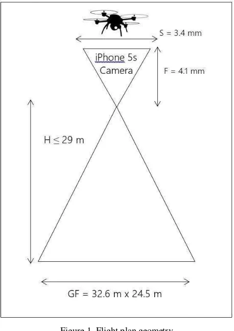
1.3 Flight Plan
GSD: 1 cm
Maximum AGL: 29 m
Desired Image Scale: 1:7,000 Ground Footprint: 32.6 m x 24.5 m
Overlap: 70%
Sidelap: 40%
Number of Flight Lines: 10
Distance Between Flight Lines: 9.8 m
Air base: 7.35 m
Image acquisition rate: 1fps Total Number of Exposures: 258
Table 1. Flight plan settings
Figure 1. Flight plan geometry
1.4 Ground Control Points
Nine ground control points (GCPs) were surveyed for accurate georeferencing by using RTK GPS. The horizontal and vertical accuracy are about 2 cm and 2cm, respectively. WGS-84 UTM Zone N10 coordinate system was chosen.
2. POINT CLOUD DATA PROCESSING 2.1 Point Cloud Processing Software
For point cloud generation, the Pix4D software was used. The Pix4D software has been widely used in the sUAS community and can process huge numbers of images into geo-referenced point clouds, digital surface models (DSMs), and orthophoto mosaic.
2.2 Processing Workflow
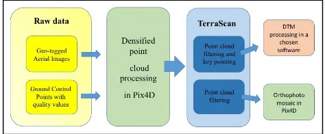
Figure 2 shows the typical input and output data of the Pix4D software. Since the user has no control on the filtering function in Pix4D, the raw “densified” point cloud was used in this investigation. Next, the noise filtering and key pointing were done in the TerraScan software. The key pointing was set to 20 cm.
Figure 2. Inputs and outputs in Pix4D
Statistics on the final point cloud is shown in the Table 2.
Number
of points Area
Point density
XY RMS error at
GCPs
Z RMS error at GCPs
[pcs] [sqm] [pnts/sqm] [m] [m]
312,473 5,133 61 0.06 0.03
Table 2. Statistics of final point cloud
3. QC ON THE POINT CLOUD 3.1 Traditional Geodetic Survey
Simultaneously with the GCP measuring, the test area was surveyed in transects, including ground, top of the cliff, bottom of the cliff, etc. The total of 141 surveyed points was classified by the following thematic:
GCPs (9) Top of cliff (54) Bottom of cliff (24) Ground (54)
3.2 List of TIN and GRID Models used for QC
A TIN model, TIN01, was generated in TerraModeler based on the key points classified from the Pix4D point cloud for numerical analysis. The workflow of producing the TIN01 is: Point cloud generated by Pix4D → Noise filtering, classification, and key pointing in TerraScan →TIN model in TerraModeler
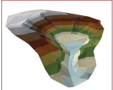
A TIN model, TIN02, was generated in ArcGIS based on the key points classified from the Pix4D point cloud for visual analysis, see Figure 3. The workflow of producing the TIN02 is: Point cloud generated by Pix4D → Noise filtering, classification, and key pointing in TerraScan →TIN model in ArcGIS
A TIN model, TIN03, was generated in ArcGIS based on the RTK GPS survey data for visual analysis, see Figure 4. The workflow of producing TIN03 is: Points from the Trimble RTK GPS → Vectorization (points and breaklines) in AutoCAD 2014 → TIN model in ArcGIS
0.4 m cell size GRID model, GRID02, was interpolated based the TIN02 using “natural neighbour” interpolation for visual analysis.
0.4 m cell size GRID model, GRID03, was interpolated based the TIN03 using “natural neighbour” interpolation for visual analysis
Figure 3. TIN03 model: based on point cloud from UAS
Figure 4. TIN02 model: measured with RTK GPS receiver
3.3 Statistical Analysis 3.3.1 Height Differences
The statistical analysis is shown in Table 3, a summary of the height differences between the 141 ground points and their projection on the TIN01 model. The projection was done in TerraModeler; note the interpolation method is not specified in the manual of the software.
Point
types Mean Maximum Minimum STD 3*STD
[m] [m] [m] [m] [m]
GCP 0.02 0.10 -0.04 0.05 0.15
Top of
cliff -0.08 0.16 -0.25 0.08 0.25
Bottom
of cliff -0.02 0.18 -0.17 0.09 0.29
Ground
shots -0.09 0.13 -0.32 0.07 0.23
All
points -0.07 0.18 -0.32 0.09 0.26 Table 3. Statistics on height differences
3.3.2 Height Differences vs. Absolute Height
Figure 5 shows the height differences with respect to absolute height. Note the trend in the plot.
Figure 5. Height differences [m] vs. absolute height [m]
3.3.3 Volume Difference
The volume calculation was done on the intersection of the TIN02 and TIN03 surfaces, using AutoCAD Civil3D software environment. The results are listed in Table 4.
Volume intersection Cu Fill Net [cu m] [cu m] [cu m]
TIN03 - TIN02 1000 821 178
Table 4. Volume calculation, TIN03 – TIN02
3.4 Visual Analysis
Figure 6. Surveyed points’ height vs. TIN01 model
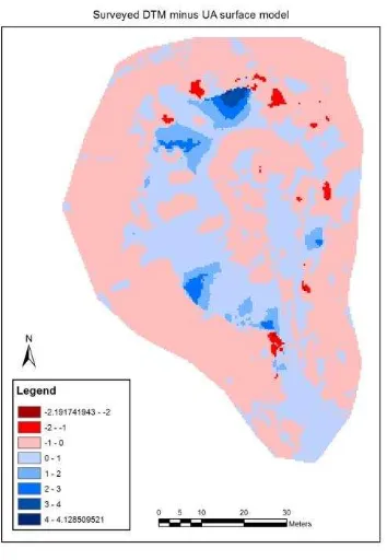
Figure 7. GRID03 – GRID02
Thematic maps help visual analysis of the height difference between the two datasets collected with different methods. Figure 6 is a visualization of the height differences between the points measured with RTK GPS and their vertical projection on the
TIN01 model. Figure 7 shows height differences between the GRID02 and GRID03.
4. INTERPRETATION OF RESULTS 4.1 The Mean Value
The mean value of height difference on all points shows a -.7 cm vertical offset. This number itself would mean that the model based on Pix4D points is shifted above the reference model.
4.2 “Height Difference vs. Absolute Height” Interpretation Almost all of the points with a positive height difference value (in other words, the height of the points projected to the TIN01 are lower than the originally measured points) are at the lower level of the test area. The regression line, marked by dotted blue in Figure 5, clearly shows this tendency; the Pix4D points at higher level are more likely above the reference model, while the Pix4D points at lower level are below the reference model.
Drawing a conclusion only from this statistical analysis would probably produce a false result, such as the model based on the Pix4D point cloud may have a vertical stretch. However, there are other environmental factors, such as vegetation, which must be considered too.
4.3 Interpretation of the “Cut” and “Fill” volume results For being able to interpret the volume values given by the differences between the TIN02 and TIN03 surfaces, the reliability of the volume calculation against the geodetic measured model must be known. Let’s consider the geodetic model (TIN03) as a reference model. A good approach is to calculate a “reliability volume” based on the confidence interval of many-repeated aerial Z measurement on a single triangle of the reference TIN model. A plane of a triangle (a triangle is considered as a plane for this model) is determined by 3 measurements. Thus, dividing the number Z measurements by three will result in the number of independent determinations of a triangle plane. This number can be considered also as many-repeated Z measurements on each single point. Using this number of independent measurements and the STD value of a single Z measurement, the 99% confidence level can be calculated. In worst-case scenario, the 3 points move in the same Z direction to the edge of the confidence interval giving the maximum volume deviation. This way, the XY projected area of a triangle and the confidence interval determine the “reliability volume” for a single triangle. Summarizing all the “triangle volumes” gives the “reliability volume” for the whole test area. Table 5 shows the results of the “reliability volume” calculation.
Number
Table 5. “Reliability volume“ calculation
Using this 99% confidence level may be too optimistic, since the RMS of the Z error at the GPCs in the Pix4D report is given as 0.03 m. Also, our statistical analysis shown in Table 3 gives a 0.05 m STD value at the GCPs. Using our STD value results 257 cu m as “reliability volume”, see Table 6.
Note that this second approach is a very conservative, since it is very unlikely to have all the points moved in the same direction;
more precisely, the chance is one to the half of the two of the power of the number of the points, which is 1:256 in this case.
Area Z STD on
Table 6. “Reliability volume“ calculation based on STD value of GCPs
Comparing the reliability volume and the “Net” volume (Table 4) given by the variety of the TIN02 and TIN03 models, we can conclude that the modeling based on UAS measurement give us, at least, as reliable volume calculation as the traditional method. However, looking at the “cut” and “fill” numbers, it is clearly seen that the UAS data describes the variety of the terrain more accurately (more detailed) than the geodetic method.
4.4 Visual Interpretation of Figure 6
Visualizing the points on the orthophoto of the test area makes the interpretation easier. The following statements and conclusions can be drawn based on Figure 6:
Most of the ground in the northern region is covered by grass. The grass has a significant impact on the height of the point cloud acquired by using imagery, clearly explaining the offset between the two method’s data and reduces the presumption of the stretching model theory.
Most of the points with positive height difference (blue dots) are in the southern area, where there is no grass. The points without the impact of grass coverage have better chance to have positive height difference; this fact, again, reduces the presumption of the stretching model theory.
The area with the points in the southern area with significant negative values (big red dots) is also covered by grass. The significant positive values in the southern area points would reduce the presumption of the stretching model theory, so to a less extent.
Most of the points with positive height difference are concentrated on a small area (on the south of the test area), and might be explained with a local anomaly, directing attention to another type of possible error of this method.
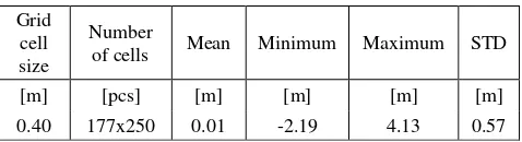
4.5 Interpretation of Figure 7 Grid
Table 7. Statistics on GRID03 – GRID02
Figure 7 visualizes the differences of the topographic variety based on the GRID02 and GRID03 surfaces. Note the high height differences at the cliff walls, which are the result of the more detailed aerial survey against the rough generalization of the geodetic survey. The statistical values of this comparison are shown on Table 7. Note the small mean value of the height
differences; it is within the accuracy level of the GCP measurement. Due to the rough generalization of the geodetic measurements, the minimum, the maximum, and the standard deviation values are relatively high.
5. CONCLUSIONS
This paper analysed the performance of a low-cost sensor and platform based solution for aerial topographic data acquisition. An iPhone 5s installed on a sUAS platform acquired imagery over complex terrain, and the Pix4D software produced the point cloud for the analysis. The test area was extensively surveyed to provide absolute control for the investigation.
The results of the performance evaluation clearly indicate that the imagery acquired by this inexpensive system is able to provide derived products that are comparable in accuracy to traditional airborne surveying performance. Thus, except for productivity, this simple system is surprisingly competitive to conventional high-performance sensor equipped airborne systems.
Despite the lower quality of the imaging sensor, due to the high redundancy of measurements, the system is capable for acquiring high detailed topographic data; in fact, the final results appear to be, at least, as reliable as the geodetic method-based reference.
During this study, various data processing methods were used, and based on this experience, the workflow, shown in Figure 7, is recommend to achieve the most reliable products, such as digital terrain model and orthophoto mosaic.
Figure 7. Recommended workflow
ACKNOWLEDGEMENTS Acknowledgements of support for Towill, Inc.
REFERENCES
Wassermann, L., 2010, All of Statistics: A Concise Course in Statistical Inference (Springer Texts in Statistics), Springer
http://iphonedroneimagery.com
http://3drobotics.com
http://www.apple.com/iphone/
http://pix4d.com
http://www.terrasolid.com/