BACKSCATTERING OF INDIVIDUAL LIDAR PULSES FROM FOREST CANOPIES
EXPLAINED BY PHOTOGRAMMETRICALLY DERIVED VEGETATION STRUCTURE
I. Korpela a, *, A. Hovi a, L. Korhonen b a
Department of Forest Sciences, POB 27, 00014 Univ. of Helsinki, Finland - (ilkka.korpela, aarne.hovi) @helsinki.fi b
School of Forest Sciences, Univ. of Eastern Finland, Joensuu, Finland - [email protected]
KEYWORDS: canopy imaging, silhouette, footprint, echo triggering, waveform LiDAR
ABSTRACT:
In recent years, airborne LiDAR sensors have shown remarkable performance in the mapping of forest vegetation. This experimental study looks at LiDAR data at the scale of individual pulses to elucidate the sources behind interpulse variation in backscattering. Close-range photogrammetry was used for obtaining the canopy reference measurements at the ratio scale. The experiments illustrated different orientation techniques in the field, LiDAR acquisitions and photogrammetry in both leaf-on and leaf-off conditions, and two-waveform recording LiDAR sensors. The intrafootprint branch silhouettes in zenith-looking images, in which the camera, footprint, and LiDAR sensor were collinear, were extracted and contrasted with LiDAR backscattering. An enhanced planimetric match (refinement of strip matching) was achieved by shifting the pulses in a strip and searching for the maximal correlation between the silhouette and LiDAR intensity. The relative silhouette explained up to 80 90% of the interpulse variation. We tested whether accounting for the Gaussian spread of intrafootprint irradiance would improve the correlations, but the effect was blurred by small-scale geometric noise. Accounting for receiver gain variations in the Leica ALS60 sensor data strengthened the dependences. The size of the vegetation objects required for triggering a LiDAR observation was analyzed. We demonstrated the use of LiDAR pulses adjacent to canopy vegetation, which did not trigger a canopy echo, for canopy mapping. Pulses not triggering an echo constitute the complement to the actual canopy. We conclude that field photogrammetry is a useful tool for mapping forest canopies from below and that quantitative analysis is feasible even at the scale of single pulses for enhanced understanding of LiDAR observations from vegetation.
1. INTRODUCTION
Airborne LiDAR data are currently used for the retrieval of different biophysical parameters in forests. Many applications use distribution metrics derived from echoes of multiple pul-ses. While the use of geometric features has been the main-stream, radiometric features are useful as well. Sensors capab-le of waveform (WF) recording have emerged, giving a better display of the volumetric backscattering in vegetation. Back-scattering of individual LiDAR pulses explained by ratio-scale vegetation characteristics have not been studied empirically. Such studies and those with simulators increase our under-standing of the LiDAR data and aid in developing more de-ductive approaches.
Airborne LiDAR is a tool for probing the vegetation and topography. It uses pulsed sensors that transmit 1 3-m-long, highly collimated, high-power monochromatic laser pulses in an identified direction from a known 3D location. The medium and targets contribute to backscattering that is received through a narrow iFOV and a spectral band-pass filter. A photon detec-tor measures the returning photon surge. The signal is proces-sed into discrete-return (DR) observations and/or quantized in-to a WF amplitude sequence. Given the known pulse vecin-tor, the ranges measured are converted to target coordinates. The actual implementation of range detection and the overall sensor functioning is often obscured from the users. The ground is essential for topographic applications, while the entire canopy-ground profile is used in the forest. LiDAR pulses map both canopy targets and gaps from the above, while transmission losses limit the most accurate potential to the dominant canopy, which is met first by the pulses.
The geometric accuracy of LiDAR data is strongly dependent on the accuracy of sensor orientation data that are required for each pulse. Interpolation of satellite positioning data and
inert-ial measurements provide direct sensor orientation. These data are corrected in postprocessing, in which hierarchical error mo-dels are fitted to redundant data. There are systematic cam-paign- and strip-level errors as well as short-term errors. Cyclic interior orientation (IO) errors, e.g. due to mirror deformations, are possible. Processed LiDAR data combine the time-stamped sensor geometry observations, including different calibrations into meaningful observations. Analyses of individual pulses re-quire very accurate geometry of both the LiDAR pulses and the reference data.
Raw LiDAR data that are comprised of time, range, and ampli-tude/intensity data may show ‘empty data’, i.e. pulses transmit-ted but not resulting in an observation, because the LiDAR ob-servations are ‘triggered’. This implies that radiometry and geometry are interconnected. Near-infrared (NIR) lasers are commonly used in topographic sensors. The signal received contains noise caused by e.g. solar illumination, internal elect-ronic noise, quantization noise, and backscattering from the medium, which explain the need to threshold. Sensor propert-ies are obscured from the users, which hinders radiometrically quantitative LiDAR remote sensing. Vicarious calibration of intensity data to target reflectance factors is feasible, using re-ference targets of known reflectance. Without calibration, it is challenging to compare the radiometry between campaigns and sensors even between DR returns in a pulse.
The exact temporal power distribution of the transmitted pulse is typically unknown. The shape can be retrieved from the WF data of well-defined surfaces. These data are influenced by the system response of the receiver (linearity, rise/fall dynamics of the photon detector and subsequent circuits, etc.). Pulses trans-mitted should exhibit minimal interpulse variation. The irradi-ance distribution across the pulse cross-section is understood to be defined by Gaussian point spread, and therefore the
scattering from a small target is dependent on the intersection geometry. The scattering in vegetation is volumetric. The geo-metry and reflectance properties of individual scatterers vary greatly, as does the incident illumination. The density and spat-ial arrangement of foliage influence the WF that returns from the vegetation, and the WF is a sum of the contributions across a volume that potentially has a larger 'diameter' than the foot-print, because of strong multiple scattering in the NIR. In some cases, scattering of the emitted photons can occur even outside the iFOV of the receiver. The radar equation states that the po-wer received (of that transmitted) is dependent on the scanning range, transmitted power, beam divergence, receiver aperture, losses in the medium, as well as the target geometry and scat-tering characteristics. The target properties are embedded in the backscattering cross-section and coefficient, which are ob-tained in calibration of the WF data by eliminating the cam-paign- and sensor-specific effects from the WF observed. The choice of appropriate calibration parameters is dependent on the target. Vegetation targets are neither well-defined surfaces nor pointlike features. Thus, both the backscattering cross-sec-tion and coefficient are affected by the beam divergence and scanning range, making the calibration íll-posed. As an examp-le, normalization for the effects of varying scanning range on intensity within a single LiDAR campaign is dependent on the tree species.
Although LiDAR observations are made in the hot-spot geometry, the intersection geometry affects the signals at the pulse level. In forest vegetation, strong backscattering is obser-ved in plants with large planophile leaves or from compact coniferous shoots. The particular traits of the LiDAR data in the vegetation are the transmission losses that skew the popu-lation of the low-canopy and ground targets that trigger an observation. A pulse intersecting a branch has less energy left on the forest floor. A surface of low reflectivity, e.g. a wet patch, may not trigger an observation, while a dry patch of fo-rest floor would. The same selection towards large, dense, and/or reflective targets also applies to low vegetation.
The objectives (research questions, RQ) of our work were
1. To examine the feasibility of close-range photogrammetry in linking individual airborne LiDAR pulses with ratio-scale vegetation characteristics.
2. To examine the dependence of the LiDAR backscattering on the intrafootprint silhouette extracted from the zenith-looking images. The radar equation states that the dependence should be strong in vegetation that displays limited and stationary variation in reflectance and surface geometry.
3. To test whether the approach can be used for detecting the minimum echo-triggering vegetation object and whether LiDAR pulses adjacent to canopy vegetation, which did not trigger a canopy echo, can also be used for the determination of the minimum object.
2. MATERIALS AND METHODS
We experimented in Hyytiälä, Finland (62ºN, 24ºE). A Li-DAR-based DEM and low-altitude LiDAR data were used to assess the terrain. Accurately oriented aerial images were avai-lable from 2006, 2010 and 2012. The images were used for measuring control points (CPs). The CPs served for the pur-pose of transforming local observations into the coordinates of the LiDAR data.
2.1 Notes on the field data and photography
Research of individual pulses calls for very accurate geometry. In forests, artificial features for geometric postprocessing of Li-DAR data are rare. Vegetation and smooth topography hampers strip matching. LiDAR data thus always display absolute and relative, constant, or time-dependent xyz errors. High accuracy is also needed for the vegetation geometry. A particular aspect is the motion due to wind as overlapping strips are acquired over periods of several minutes. Geodetic GNSS provides cen-timeter accuracy in open areas, but is less accurate under an obstructing canopy. Mapping of local vegetation details calls for indirect methods: resection with a theodolite or a camera or direct observations with a terrestrial laser scanner (TLS).
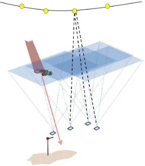
The actual implementation of our field activities varied bet-ween sites. The idea was to take vertical images at locations in which the pulse or its extension had traversed (Fig. 1). In such images, the projection of the pulse ray, after some distance from the camera, becomes a point and the footprint is circular, enabling the measurement of the silhouette area of the branch-es intersected by the pulse. We aimed at accurate orientation of the cameras. This comprised the IO and the exterior orientation (EO) in the coordinate system of the LiDAR data. The EO of the image blocks was solved, using bundle block adjustment in two phases.
Figure 1. An illustration of the preferred pulse-camera geomet-ry. The leftmost camera is adjacent to the pulse path with its optical axis pointed towards the zenith. The camera was attach-ed to a monopod with a ball joint mount. The dashattach-ed lines dep-ict ray intersection to tie points, which were natural or artific-ial, as depicted here.
All images were taken with a 1.5-m-high leveled monopod, which had a ball joint mount of known radius. The 3D offset of the camera projection center was estimated. The images were taken from marked locations that were positioned with a total station. The transformation to the coordinate system of the Li-DAR data involved estimation of the rotation about the z axis as well as the offsets in x, y, and z. The photographs were taken in calm wind, against a clear sky, and when the sun was low. We used a Canon Powershot G6 and a Nikon D300 at the minimal focal length, 7 and 18 mm, respectively. The cameras were calibrated prior to and after the photography, using iWitness. The G6 was sensitive to the F number, and we noted a 0.5% change in the camera constant between F values of 2 and 4.
2.2 Close-range photogrammetry at four sites
In June 2011, we attempted to 'position the pulses' in a mature pine stand, using backward trilateration and triangulation. The trunks were the xy CPs. Their positions were obtained by map-ping the treetops in aerial images. Selected LiDAR pulses of 2010 (Table 1) were solved for the xy coordinates 1.5 m above the ground. These camera locations were positioned with a to-tal station. The local coordinate system was transformed into the coordinate system of LiDAR data, using trilateration and triangulation to the CPs. The RMS of the xy residuals was 7 cm. The xy accuracy may include systematic errors, due to the photogrammetric treetop positioning. We had polystyrene sphe-res (CPs) in the canopy for the control of systematic errors in camera IO. Photography was performed, when the trees had needles formed in 2010, 2009, and some in 2008.
In May 2012, we did leaf-off photography of semi-urban trees. Because of the good visibility, we could orientate the total sta-tion, using artificial targets that were positioned in aerial ima-ges. The xy position of the total station was achieved at sdevs of 3 6 cm.
In June 21 and July 6, 2012, two 12 10-m plots (pine and spr-uce) were photographed in a 1-m grid, giving 143 images (Fig. 1). Again, interpoint distance and azimuth observations to trees were used to establish the orientation. A precision of 0.05 m was achieved on both plots. The pines were 12 19 m high and the visibility was better than in the spruce stand. The stem density was 800 per ha and the pine crowns were relatively short, with the lowest living branches at 11 m. The spruce plot was comprised of 16 24-m-high trees, forming a very dense canopy with deep crowns. Finding natural tie points was im-possible in the spruce canopy and we resorted to artificial tie points. The pines had needles from 2012, 2011, 2010 and some from the cohort of 2009. The spruces had on average six needle cohorts.
2.3 Block triangulation
We used iWitness, which utilizes the principle of relative orie-ntation. The relative solution obtained was brought to the right scale, orientation, and position using a 3D similarity transfor-mation. We supplied xyz coordinates of tie points or the came-ra projection centers. The latter had an estimated accucame-racy of about 8 12 mm. The RMS of the image residuals was 2 3 pi-xels. We refined this solution by performing a weighted least-square adjustment, using the image observations and 3D coor-dinates of the CPs and projection centers.. The average a poste-riori sdevs of the camera positions were 4 7 mm.
2.4 Airborne LiDAR data
We utilized four WF campaigns acquired in 2010 2012 (Table 1). All but the leaf-off data of 2011b included several flying altitudes. ALS60 sensors were used for the leaf-on acquisit-ions, while an LMS-Q680i was used for the leaf-off data. The strip overlaps were 20 85%. In 2012, the transmitted power was set to yield a constant SNR across the acquisition heights. The ALS60 and LMS-Q680i differ in beam divergence (0.22 vs. 0.5 mrad at 1/e2), mirror type (oscillating vs. rotating poly-gonal), echo retrieval (on-the-fly vs. postprocessing), WF re-cording (one fixed length record vs. several; triggered once vs. multiple WF samples), availability of a sample of the emitted
pulse, transmitting power (5-km vs. 3-km maximum range), adjustment of maximal scan angles (continuous 37.5º vs. fi-xed at 22.5º or 30º) and laser wavelength (1064 vs. 1550 nm).
Property Campaign
2010 2011a 2011b 2012
Sensor ALS60 ALS60
LMS-Q680i ALS60 Date,
time (GMT)
19.7., 15 18
2.8., 16 19
15.11., 15 18
5.7., 19 22
Scan angle 15º 15º 30º 15º
Range, km 1.2, 2, 3 0.75, 2 0.75 0.5, 1, 2, 2.75 Footprint,
cm (1/e2) 26, 44, 66 17, 44 38
11, 22, 44, 60
PRF, kHz 173,119,
83 118,118 240
152,99, 59,45 Table 1. Characteristics of the LiDAR acquisitions.
The summer acquisitions were all in the early evening, which is preferable, since the clouds vanish, there is yet no dew and gusts decrease. We had access to 30-s averaged observations of an anemometer 33 m above the ground. Gusts showed up in the data as short-term variations; 2 8 m/s in 2010, 1 2 m/s in 2012, 0.5 2 m/s in 2011a, and 1 2 m/s in 2011b. The tops of 15 25-m-high dominant trees swayed 10 20 cm at wind speeds of 1 3 m/s. We concluded that the 2010 campaign dif-fers significantly from the others.
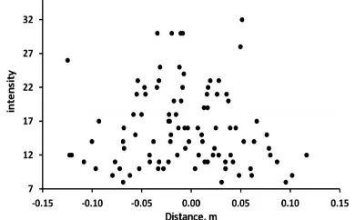
Figure 2. Intensity of LMS-Q680i (dataset 2011b) echoes trig-gered by 40-m-long power line cables. Horizontal axis shows the distance from the cable. The within-pulse irradiance is the-oretically Gaussian.
We checked the z and xy accuracy, using road surfaces and borderlines that showed abrupt reflectance or geometric chan-ges and concluded that all LiDAR data were within 25 cm in xy and 5 cm in z. Figure 2 shows an example in which the first echoes from power line cables that run parallel to the flight path. Perfect pulse geometry, stationary reflectance of the cab-le, and a Gaussian intrafootprint irradiance variation would re-sult in a bell-shaped intensity pattern. We can assume that the cable triggered WF recording only if it was intersected by the center of the footprint ± some interval. If the interval was ± 5 cm, the pattern was reproduced by simulating the geometric error to have an sdev of 5 cm. This would, constrained by the assumptions made, be the noise in the direction of the scan pat-tern, in a single strip, and from a height of 750 m.
2.5 Radiometry of the LiDAR datasets
The ALS60 receivers were operated with the automatic gain control (AGC) switched on. The AGC effects need to be remo-ved from the intensity and WF data. We used intensity norma-lization models fitted to data from homogenous surfaces of var-ying : bitumen, 0.05; old asphalt, 0.16; fine dry sand, 0.30; grass, 0.45. Within a surface, the dependence between gain and the backscatter strength was linear, motivating the choice of model, which assumes that the signal through the AGC cir-cuit is unaltered at some reference gain value a, and the ampli-fication factor b is constant.
Ical = Iobs / ((agc a) b + 1) (1)
The (case-specific) parameters a and b were found by maximi-zing the total decrease in intraclass coefficients of variation by observing the remaining trends. The modeling was done sepa-rately for each acquisition height as well as for the intensity and WF amplitude data, except in 2012 (constant SNR). The LMS-Q680i scanner has a fixed receiver gain. Some Q680i pulses produced up to 10 echoes, implying high sensitivity. The short pulses improve the range resolution. The WF samp-ling rate was 1 ns in all datasets.
2.6 Analyses of LiDAR pulses in canopy images
In this phase, the EO accuracy of each internally accurate image block was 5 10 cm and that of the pulse paths 25 cm or better in the object space. The data were filtered for pulses that were ‘viewed by an image from their tail’. The pulses needed to be adjacent to the camera (Fig. 1). We then manually select-ed cases in which the branch triggering the first echo was ‘appropriate’. The 1/e2 footprint was projected onto the image. Subjective assessment followed. Branches that were viewed without occlusions and had a clear background were ideal (Fig. 3). In accepted cases, the first echo was shifted, with x and y taking values at 0.05-m intervals to examine the best planimetric match between the pulses in a strip and the field data (Fig. 4). The subimages of the shifted footprints were extracted and image binarization was done in the 8-bit blue channel, using a series of threshold (th) values. The relative silhouette areas (0 1) were computed by weighting the scat-terer pixels with Gaussian and constant irradiance trend across the footprints (Fig. 7).
Correlations were then computed between the silhouette and the backscattering variables, which were the maximum ampli-tude and the DR intensity. The maximum correlation in the ( x, y, th) grid was searched, and the ( x, y)| rma x values were a fine-tuning of strip adjustment (Fig. 4). This additional ‘local strip-adjustment’ was only done in strips that provided eight or more observations. Some 2011b data were omitted, because the scan zenith angles exceeded the FOV of our cameras.
2.7 Use of pseudoechoes
Because LiDAR pulses also measure canopy gaps, we verified the ( x, y)-adjusted pulse geometry, using ‘pseudoechoes’. They are footprints of pulses that are back-projected to an elevation (z) along the pulse path (Fig. 5). The images enabled 3D positioning of branches and the pseudoechoes could be de-fined at the elevation of these. This allows a selection of pulses
adjacent to canopy vegetation that did not trigger a canopy echo. If the overall geometric match of the LiDAR and photo-grammetric data is favorable, and the geometric precision of the pulses (cf. Fig. 2) and the orientation of the individual ima-ges is high, such pseudoechoes should show no or minimal sil-houette area.
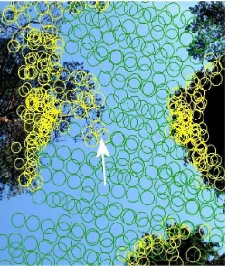
Figure 3. Relative footprint silhouette was extracted in images for detached branches inside a 1/e2 footprint image that was binarized Leica ALS60 pulse with a 256-sample waveform, transmitted from a height of 2100 m. The pine branch is 15 m above ground and is the first target intersected by the pulse.
Figure 4. The correlation (y-axis) between the silhouette and backscattering intensity was examined by shifting the reference data in XY. Strip-level errors XY were eliminated, using this approach.
Figure 5. Pseudoechoes (green) at z = 158.69 m and real ec-hoes (yellow) superimposed in an image. The tip of the pine shoot in the center was measured to be at that elevation.
3. RESULTS
3.1 Silhouette analyses in pulses viewed collinearly
The silhouette area explained up to 80 90% of the between-pulse variance in the strength of backscattering (examples in Figs. 6 and 7, Table 2). However, accounting for the within-footprint Gaussian spread of irradiance did not increase correlations in any of the datasets. The fitted lines in Fig. 6 suggest that the LMS-Q680i sensor was more sensitive. However, accounting for the differences in the footprint area (3:1), a smaller object triggered an echo in the ALS60. The transmitting power was limited in the low-altitude ALS60 data of 2012 to assure constant SNR. The SNR was thus set by the highest 2.75-km acquisition.
Figure 6. Dependence between non-weighted relative silhoue-tte area and the intensity of the first echo in pine shoots for 1 km Riegl (38 cm footprint) and Leica (26 cm) data.
Campaign, acquisition height [m], strip code
N
Pulse zenith angle [º]
x, y [m]
Correlation
coefficient
2012, 500, 1 10 9
15 0.05, +0.20
0.572 2012, 500, 2 11
3
15 +0.10,+0.0 5
0.725 2012, 1000, 1 51 13 +0.05,+0.1
5
0.840 2012, 1000, 2 48 9 +0.00,
+0.00
0.732 2012, 2000, 1 12 9 +0.20,+0.2
0
0.936 2012, 2000, 2 13 7 0.05,
+0.15
0.950 2012, 2000, 3 26 14 +0.00,
0.05
0.755 2012, 2000, 4 19 7 +0.10,+0.1
0
0.919 2011a, 700, 5 70 6 +0.05,
+0.15
0.707 2011a, 700, 6 94 13 +0.00,+0.2
0
0.667 2011a, 2000, 1 11 8 +0.05,+0.0
0
0.763 2011b, 750, 1 91 10 -0.05,+0.10 0.639 Table 2. Best case correlation between the silhouette area (Gaussian weighting of scatterer pixels) and first-return intens-ity in the 60-yr-old pine stand. N is the number of silhouettes and ( x, y [m]) is the optimal xy offset. Gain normalization (1) is applied to the ALS60 data.
The AGC correction increased the correlations in the ALS60 data (2012 and 2011a), and the effect was strongest in the lowest acquisitions, where the gain had varied most.
3.2 Pseudoecho analyses
The pseudoechoes preceded the first real echo, so we did not assess the transmission losses from the silhouettes between
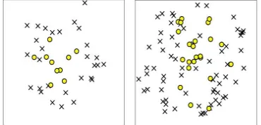
ec-hoes. Fig. 8 shows the results. Assuming perfect pulse geo-metry and image orientation there should be no pseudoechoes close to the branch tip. The closest ALS60 pseudoechoes were 4 cm from the branch and that the proximate pseudoechoes had positive silhouettes. The same is shown for the Riegl data, which also appear to be asymmetric in the xy. This analysis ve-rified that the LiDAR and/or image data had small-scale geo-metric errors.
Figure 7. Examples of LMS-Q680i (1/e2) first-echo footprints in pine crowns, showing an intensity gradient with DN values of 10, 15, 26, 37, 46, and 89. The largest value is associated to a single echo, while the rest are of type first-of-many.
Figure 8. The xy offsets to the positioned branch tips from the centers of the pseudoechoes that had zero (x) or positive (o) silhouette. The scales differ: left subfigure shows the 1-km ALS60 strip in a ± 30-cm box and the right subfigure shows the offsets in the Riegl 750-m LMS-Q680i data in a ± 50-cm box.
Figure. 9. A 2011b pulse intersecting an aspen branch. The oblique image pair views the targets from a 20-m distance with a baseline of 5 m. Amplitude values at 1-ns sampling are su-perimposed as dots coded in grayscale. The arrows depict the first and second echoes. Such oblique images and those collinear with the pulse help clarify, which targets contribute to the backscattering. A sphere (CP) is shown in the foreground.
3.3 Qualitative observations
After the xy offsets were solved for the strips, we selected pul-ses that traversed very close to a camera. Projecting the pulse
path in overlapping (~stereo) images could be used for de-termining which branches, shoots, or stem parts contributed to the backscattering (e.g. Fig. 9).
4. DISCUSSION AND CONCLUSIONS
4.1 Feasibility of the photogrammetric approach (RQ 1)
Our experiment was mostly successful, but there remains room for improvement. The absolute xyz geometry of the image blocks could be established, using more accurate CPs than those measured in aerial images. Establishing an internally accurate image block was challenging under a dense canopy and we even resorted to artificial tie points. We used iWitness for calibration, relative orientation, and for the 3D transformation of the images to the coordinates of the LiDAR data. iWitness did not provide the standard errors of the calibration parameters and we needed to carry out a separate weighted least-square adjustment to consider differences in the observation accuracies. The use of terrestrial laser scanning (TLS) is an alternative. However, many scan positions are nee-ded to overcome the problems of occlusion. The same chal-lenges of accurately transforming the local coordinates to those of the LiDAR remain with TLS.
4.2 LiDAR backscattering in vegetation (RQs 2 and 3)
The correlation analyses verified the assumption that the silhouette area is a major factor explaining the strength of the backscattering in the case of homogenous-stationary target reflectance and geometry. We hypothesized that accounting for the Gaussian spread of intrafootprint irradiance would improve the correlations, but the remaining geometric inaccuracies were the likely cause for not being able to verify the thesis in situ. In addition, multiple scattering certainly causes an averaging ef-fect. We showed that rather small targets that intersect only a small portion of the footprint can produce an echo or initiate WF recording. However, the remaining geometric inaccuracies prevented us from carrying out exact analyses of the required target size. A particular challenge in the estimation of the cor-rect silhouette area, or related variables such as the canopy co-ver or the leaf area index (LAI), is in the image binarization task. Previous studies and our experiments have shown that results are influenced by the selection of the threshold. We showed that even individual branches can be used as mo-numents for local fine-tuning of the LiDAR geometry. We also had fair evidence that tree sway due to wind worsened the re-sults. While carrying out the selection of pulses by visual as-sessment, it was sometimes very interesting to be able to ‘see’ that a single pulse had a ‘dampening WF tail’ caused by dead branches and twigs in the volume of the pulse path. Future work is needed in analyzing the WF data for potential species-specific features that would be useful for enhanced tree species discrimination, which constitutes a bottleneck in LiDAR-based forest applications.
4.3 Other potential uses of the approach
Determination of the silhouette area from the intensity data is especially useful in the estimation of vegetation cover and LAI, which are linked with the silhouette. For range detection ana-lyses, it would be vital that the absolute EO of the photogram-metric data be very accurate. The pseudoechoes and adjacent pulses that complete echo-triggering pulses and measure ca-nopy gaps could be useful in object delineation algorithms that
normally use the real echoes only. Examples include tree de-tection algorithms, while others could be found in non-forest applications as well. The strategy of the algorithms needs to be adjusted to utilize the adjacent pulses.
4.4 Conclusions
Our study illustrated some of the sources of variation in the backscattering of individual LiDAR pulses in forest canopies. We confined mostly to first echoes of multiecho pulses at crown edges that we could view against a clear background in the vertical images taken from the ground. They are only a small subset of pulses reflecting from tree crowns. The main conclusion of our work is that the silhouette area explains a large degree of the intensity variation in individual branches. We could not verify, using the field experimentation, that the intrafootprint irradiance distribution is Gaussian. The photogr-ammetric approach that we demonstrated was able to provide ratio-scale measurements of the canopy that were positioned at accuracies of about 5 10 cm. The method could also serve other research needs in the study of LiDAR-vegetation interactions.
REFERENCES
Baltsavias, E.P., 1999. Airborne laser scanning: basic relations and formulas, ISPRS JPRS 54 (2–3), pp. 199–214.
Doneus, M., Briese, C., and Studnicka, N., 2010. Analysis of full-waveform ALS data by simultaneously acquired TLS data: Towards an advanced DTM generation in wooded areas. IARPS 38 (7B), pp. 193–198.
Fraser, C., Al-Ajlouni. S., 2006. Zoom-dependent camera cali-bration in digital close-range photogrammetry. PERS 72 (9), pp. 1017 2016.
Korpela, I., Ørka, H. O., Heikkinen, V., Tokola, T., and Hyyp-pä, J., 2010. Range- and AGC normalization of LIDAR intensi-ty data for vegetation classification. ISPRS JPRS 65 (4), pp. 369 379.
Korpela, I., Hovi, A., and Morsdorf, F., 2012. Understory trees in airborne LiDAR data - Selective mapping due to transmiss-ion losses and echo-triggering mechanisms. RSE 119, pp. 92– 104.
Schenk, T., Seo, S., and Csathó, B., 2001. Accuracy study of airborne laser scanning data with photogrammetry. IAPRS 34 (W4), 6 p.
Wagner, W., Ullrich, A., Melzer, T., Briese, C., and Kraus, K., 2004. From single-pulse to full-waveform airborne laser scan-ners: potential and practical challenges. IAPRS 35 (B3), pp. 201–206.
Wagner, W., Ullrich, A., Ducic, V., Melzer, T., and Studnicka, N., 2006. Gaussian decomposition and calibration of a novel small-footprint full-waveform digitising airborne laser scanner. ISPRS JPRS 60 (2), pp. 100–112.
Wagner, W., 2010. Radiometric calibration of small-footprint full-waveform airborne laser scanner measurements: Basic physical concepts. ISPRS JPRS 65 (6), pp. 505 513.