Spectral tests of the martingale hypothesis
under conditional heteroscedasticity
Rohit S. Deo
*
New York University, 8-57 KMEC, 44, West 4th Street, NY 10012, USA
Abstract
We study the asymptotic distribution of the sample standardized spectral distribution function when the observed series is a conditionally heteroscedastic martingale di!er-ence. We show that the asymptotic distribution is no longer a Brownian bridge but another Gaussian process. Furthermore, this limiting process depends on the covariance structure of the second moments of the series. We show that this causes test statistics based on the sample spectral distribution, such as the CrameHr von-Mises statistic, to have heavily right skewed distributions, which will lead to over-rejection of the martingale hypothesis in favour of mean reversion. A non-parametric correction to the test statistics is proposed to account for the conditional heteroscedasticity. We demonstrate that the corrected version of the CrameHr von-Mises statistic has the usual limiting distribution which would be obtained in the absence of conditional heteroscedasticity. We also present Monte Carlo results on the "nite sample distributions of uncorrected and corrected versions of the CrameHr von-Mises statistic. Our simulation results show that this statistic can provide signi"cant gains in power over the Box}Ljung}Pierce statistic against long-memory alternatives. An empirical application to stock returns is also provided. ( 2000 Elsevier Science S.A. All rights reserved.
JEL classixcation: C12
Keywords: Sample spectral distribution function; Martingale di!erence; Conditional heteroscedasticity; CrameHr von-Mises statistic
*Tel.:#1-212-998-0469; fax:#1-212-995-4003. E-mail address:[email protected] (R.S. Deo).
1. Introduction
Economic theory suggests that many"nancial and economic time series like stock returns and exchange rate returns are uncorrelated. More speci"cally, the concept of market e$ciency leads one to believe that future values of such series should be unpredictable given the past. This is the famous martingale di!erence hypothesis and it is a more serious restriction than mere absence of correlation. It implies that there is no non-trivial function of past data, linear or non-linear, which can be used to predict future values. Testing such a general hypothesis is however practically impossible, since it encompasses too many possibilities. A more realistic approach towards testing the martingale hypothesis has been through testing for the absence of correlation under various data-generating mechanisms.
Two popular tests for uncorrelatedness are the variance ratio test of Cochrane (1988) and the spectral based tests of Durlauf (1991). The spectral-based tests exploit the fact that under the null hypothesis of a martingale di!erence, the spectral distribution function is a straight line. Thus, deviations of the sample spectral distribution from the straight line may be used to test for the presence of correlation. Durlauf showed that under the null hypothesis of a martingale di!erence, a normalized version of the di!erence between the sample and theoretical standardized spectral distribution function converges to a Gaussian process. The asymptotic distributions of various functionals of this di!erence can then be obtained and tests for departure from the null of no correlation may be obtained. Durlauf (1991) obtained his limiting distribution under conditions which ruled out conditional heteroscedasticity. However, it is a well-accepted fact that most "nancial and economic series which are hypothesized to be martingale di!erences show conditional hetero-scedasticity. Thus, it is important to take this conditional heteroscedasticity into account when studying the behaviour of the spectral-based tests of the martin-gale di!erence hypothesis.
In this paper, we show that the spectral-based tests no longer have the usual limiting distribution when there is conditional heteroscedasticity. As a matter of fact, we show that, in general, the limiting distribution is heavily right skewed, with the amount of skewness depending on the degree of persistence in the second moments. This fact may explain why such tests tend to reject the martingale di!erence null in favour of mean reversion. We also suggest a way to correct these tests in a non-parametric way to account for the conditional heteroscedasticity. For one such corrected test, we prove that the asymptotic distribution is the same as what would be obtained in the absence of conditional heteroscedasticity. We provide Monte Carlo simulations for some of the uncor-rected and coruncor-rected tests and also provide an empirical application.
assumptions. In Section 3, we derive the limiting distributions of spectral-based tests for the martingale di!erence hypothesis. Modi"ed versions of the test statistics to account for the conditional heteroscedasticity are proposed and the limiting distribution for one of the modi"ed test statistics is obtained. In Section 4, we present Monte Carlo simulation results for some of the uncorrected and corrected test statistics and in Section 5 apply these tests to real data. We"nish the paper with a technical appendix containing the proofs of all our results.
2. Assumptions
We will derive the limiting behaviour of various spectral distribution tests under the hypothesis that the time series of interest,X
t, satis"es X
t"k#et, (1)
whereMetNis a martingale di!erence sequence andkis some real number. Thus,
X
t may be the "rst di!erence of a random walk with martingale di!erence
innovations. Our speci"cation allows the random walk to have a possible drift, implying a non-zero mean for the observed seriesX
t. The assumptions we make
about the martingale di!erence seriesMetNin (1) are as follows:
Condition A. (i) E(e
tDFt~1)"0, whereFt~1"pMet~1, et~2,2Nis the sigma
"eld generated by Me
t~1, et~2,2N.
(ii) E(e2
t)"p2(R.
(iii) lim
n?=n~1+nj/1E(ej2DFj~1)"p2'0 almost surely.
(iv) There exists a random variable ; with E(;4)(R such that P(DetD'u))cP(D;D'u) for some 0(c(Rand allt, allu*0.
(v) E(e2tet~ret~s)"p4q
rsis"nite and uniformly bounded for allt, r*1,s*1.
(vi) lim
n?=n~1+nt/1et~ret~sE(e2tDFt~1)"p4qrs almost surely for any r*1,
s*1.
(vii) For any integer q, 2)q)8, and for q non-negative integers
s
i, E(<qi/1estii)"0 when at least onesi is exactly one and+qi/1si)8.
(viii) E(e8
t) is uniformly bounded for allt.
The following two lemmas assert that two major models of conditionally heteroscedastic martingale di!erences, viz. the stochastic volatility model and the generalized autoregressive conditionally heteroscedastic (GARCH) model, satisfy the assumptions of Condition A. The proofs of the lemmas are in the technical appendix at the end.
Lemma 1. Let the seriesMetNbe generated by the stochasticvolatility model
et"v
texp(ht), (2)
whereMv
tNis an independent(0,p2v)stationary series, MhtNis a stationary zero mean Gaussian series andMv
tNandMhtNare independent. Assume thatE(v8t)(R.Then MetNsatisxes the assumptions of Condition A.
See Shephard (1996) for a discussion of the model (2) and its applications. Our next lemma asserts that under some conditions the GARCH(1, 1) family of models also satis"es Condition A. We have restricted attention to the GARCH(1, 1) case for simplicity of exposition. The validity of Condition A for a general GARCH(p,q) model can be demonstrated along similar lines by referring to the work of Bougerol and Picard (1992).
Lemma 2. Let the seriesMetNbe aGARCH(1, 1)process given by
et"p
tvt, (3)
wherep2
t"u#bp2t~1#ae2t~1 andMvtN is a sequence of independent standard
normalvariables. Letu'0,b*0anda'0.Furthermore,let aandbbe such thatEMlog
%(b#av2t)N(0 and EM(b#av2t)4N(1.ThenMetNsatisxes the assump-tions of Condition A.
The condition EMlog
%(b#av2t)N(0 in Lemma 2 is satis"ed by any pair (a, b)
in the set S"M(a,b):a#b(1N (see Nelson, 1990) while the condition EM(b#av2
t)4N(1 will be satis"ed by some non-empty subset ofS. For example,
values of a,b extremely close to the origin will certainly satisfy the second condition.
Assumption (viii) of Condition A, requiring the existence of at least eight moments for the martingale di!erence seriesMe
tNmight seem strong considering
that"nancial and economic series seem to exhibit thick tails. However, we feel that this assumption is essential to obtain a functional limit theorem for the sample spectral distribution function in a random function space. Furthermore, the existence of the eighth moment is not too restrictive if one can "nd a transformation g()) such that rt"g(et) satis"es Condition A when MetN itself
has only a "nite fourth moment. In such a situation, our results would then apply to the series Mr
transformation, suggested by one of the referees, is
r
t"DetD1@2sign(et). (4)
SupposingMetNwere generated by the stochastic volatility model (2), whereMv tN
has a distribution which is symmetric around zero with only fourth moment
"nite. Then, by arguments similar to those used for Lemma 1, one can show that
Mr
tTo obtain our main results on the sample spectral distribution function of theNde"ned by (4) would satisfy Condition A.
processMX
tN, we need to know the limiting distribution of the sample
autocorre-lations of MXtN. This is stated in the following theorem which follows directly from Theorem 2 of Hannan and Heyde (1972).
Theorem 2.1. Let assumptions(i)}(vii)of Condition A hold. Dexne
XM "n~1+n
t/1
X t,
p(2"n~1+n
t/1
(X t!XM )2 and
o(
i"n~1p(~2
n~i
+
t/1
(X
t!XM )(Xt`i!XM ), i*1. (5)
Then,for anyxnitexxed positive integerk, we have
n1@2q(PD N(0,W),
whereq("(o(
1,o(2,2, o(k)@andW"[wij]is ak]kdiagonal matrix withwii"qii.
It should be noted that the normalized sample autocorrelations are not identically distributed under Condition A. Their asymptotic variance depends on the covariance in the second moments of the seriesMetNat the appropriate lag. For example, under the stochastic volatility model in (2), it can be easily shown that q
ii"expM4Cov(ht, ht~i)N. Since there is no natural bound on the
covariance of a stationary series, this implies thatq
ii(and hence the variance of o(
i) can be arbitrarily large under such a model. This anomalous behaviour of the
sample autocorrelations arises due to the conditional heteroscedasticity that we are allowing in the series. The normalized sample autocorrelations will however have an asymptotic variance of 1 at all lags if the series MetNhas a constant conditional variance. This can be seen from the fact that in such a case,
qii"p~4E(e2
Furthermore, it should also be noted that the asymptotic independence of (o(
r,o(s) for anyr's'0 in Theorem 2.1 is entirely due to assumption (vii) of
Condition A. This assumption implies thatqrs"p~4E(e2
tet~ret~s)"0 for any
r's'0.
It is of interest to compare our Condition A and Theorem 2.1 with analogous assumptions and results in the seminal work of Durlauf (1991) regarding the sample spectral distribution function. The assumptions made in Durlauf (1991) are stated in his De"nition 2.1. Durlauf's assumptions are identical to our assumptions (i)}(vi) and assumption (viii) of Condition A, and hence allow for conditional heteroscedasticity. Durlauf then states his Theorem 2.1, quoting Theorem 2 of Hannan and Heyde (1972), that the normalized sample autocorre-lations ofMX
tNare both asymptotically independent and identically distributed
with unit asymptotic variance at any lag. This application of Hannan and Heyde (1972) is incorrect. As demonstrated above, the sample correlations have vari-ance depending on qii in the presence of conditional heteroscedasticity and hence are not identically distributed. Furthermore, since Durlauf (1991) does not make any assumption similar to our assumption (vii) (which implies that E(e2
tet~ret~s)"0 for any r's'0), there is no guarantee that the sample
correlations are asymptotically independent. Hence, the main results on the sample spectral distribution that Durlauf (1991) obtains in his Theorem 2.2 and subsequent Corollaries, which depend on his De"nition 2.1 and Theorem 2.1, would not hold either in the presence of conditional heteroscedasticity or the absence of some restricted form of `independencea as de"ned through our assumption (vii).
We would also like to point out that our Theorem 2.1 requires assumption (vii) in Condition A to hold only for anyq)4. However, the stronger require-ment that it hold for anyq)8 is essential in showing the tightness of the sample spectral distribution function to obtain our main result below.
In the next section, we study the asymptotic behaviour of the sample spectral distribution function in the presence of conditional heteroscedasticity. Our approach draws heavily on the work of Durlauf (1991).
3. Spectral-based tests of the martingale di4erence hypothesis
The correlation structure of a stationary time series is determined by its standardized spectral density de"ned by
f(j)"(2p)~1 +=
h/~=
ohcosjh, !p)j)p,
where oh is its correlation function at lag h. This theoretical standardized spectral density can be estimated based on the observed dataX
the sample standardized spectral density given by
an appropriate sequence of weights symmetric about zero withw
n(0)"1. If the
form of the standardized spectral density functionf(j) has been speci"ed, then departures from it can be detected by studying the normalized cumulated deviations given by
Under some conditions on the weight sequencew
n()) and assuming thatMetNis
a zero mean independent series, the result of Durlauf (1991) shows that;
n,w(t)
converges to a Brownian bridge. This result can then be used to obtain the limiting distributions of common goodness-of-"t test statistics like the CrameHr von-Mises statistic, the Anderson Darling statistic, etc., which are all functionals of;
n,w(t).
In this section, we show that when MetN is a conditionally heteroscedastic martingale di!erence,;
n,w(t) no longer converges to a Brownian bridge but to
another Gaussian process. To gain more insight into why this happens, we observe that under the null hypothesis of a martingale di!erence, all the correlations are zero and the standardized spectral density reduces to (2p)~1. Thus, the normalized cumulated deviations reduce to
;
When MXtNis a conditionally homoscedastic martingale di!erence, we know thatn1@2o(
jhas asymptotically the same distribution as the sequenceMgjN, where
which is a Brownian bridge. This result breaks down when the sample cor-relations are asymptotically heteroscedastic, as happens in the case of a condi-tionally heteroscedastic series MetN, yielding a di!erent limiting process for
;
n,w(t). The new limiting process is given in the following Theorem. Henceforth,
we will always assume that;
n,w(t) is given by (8). i.e. under the null hypothesis of
a martingale di!erence.
Theorem 3.1. Assume Condition A holds. Furthermore,let the sequence of weights w
n())satisfy the following conditions:
(i) w
Note that the limiting distribution is invariant to the choice of the weight sequencew
n()), since its e!ect washes out asymptotically. Thus, the choice of the
weights only a!ects the small sample behaviour of ;
n,w and of any statistic
depending on;
n,w.
On applying the continuous mapping theorem, we get the limiting distribu-tions of various common spectral shape tests, which we state in the following Corollary.
Corollary 3.2. Under the assumptions of Theorem 3.1, we have
(i) Anderson darling statistic
(ii) Crame&rvon-Mises statistic
(iii) Kolmogorov}Smirnovstatistic
From Corollary 3.2, it is clear that the distributions of the various test statistics depend crucially on the sequence Mq
iiN which is a measure of the
dependence in the second moments of the seriesMX
tN. As mentioned earlier, for
the stochastic volatility model in (2), it can be easily shown that q
ii"
expM4Cov(h
t, ht~i)N. If the seriesMhtNis such thatCov(ht, ht~i) is positive, then
the asymptotic variance of Jno(
i will actually be bigger than 1, which is the
asymptotic variance in the absence of conditional heteroscedasticity. To see the e!ect this has on the spectral-distribution-based test statistics, it is instructive to consider an alternative expression for one of them, the CrameHr von-Mises statistic. Whenw
n()),1, it is known (see for e.g., Anderson and You, 1996) that
the CrameHr von-Mises statistic can also be written as
C<M
i is bigger than 1, it is clear that the asymptotic
distribu-tion of C<M
n will have a thicker right tail compared to that of the usual
distribution obtained in the absence of conditional heteroscedasticity. Further-more, it is also clear that the rate of decay ofCov(h
t, ht~i) to zero (and thus that
ofqii to 1) will a!ect the thickness of the right tail, with a slower rate of decay leading to a thicker tail. Hence, using the usual cuto! points of the CrameHr von-Mises statistic will lead to over-rejection of the martingale di!erence hy-pothesis in martingale di!erence series which show strong persistence in their second moments.
The other three test statistics in Corollary 3.2 also have distributions with thicker right tails under conditional heteroscedasticity due to the in#ated variance of ;
n,w(t). The right tail of the limiting distribution of the Anderson
Darling statistic is a!ected even more seriously than the CrameHr von-Mises statistic by conditional heteroscedasticity. This is due to the fact that in the Anderson Darling statistic, the quantity ;2
n,w(t), which has a larger variance
whenqii'1, is weighted by [t(1!t)]~1which gets large for values oftnear 0 and 1.
the true parameters of the underlying process, making these tests infeasible from the practical point of view. To avoid this problem, we suggest the following non-parametric correction to the test statistics. To circumvent the dependence onqii, we work with the following modi"ed form of;
n,w(t), given by
In the proof of Theorem 3.3 below, we prove that for "xed j,
p(2[(n!j)~1+nt/1~j(X
t!XM )2(Xt`j!XM )2]~1@2is a consistent estimator ofq~1@2jj .
It then follows from Theorem 2.1 that for any"nitek, the collection of random variables (a(
1, a(2,2, a(k)@will be asymptotically independent and normal with
zero mean and variance 1. Hence, we should expect the test statistics given in Corollary 3.2 but based on;
n,w,C(t) to have the same limiting distributions as
would be obtained if MX
tN were an independent identically distributed white
noise series. This will allow us to use tabulated critical values (see Anderson and You, 1996) of the standard limiting distributions when carrying out tests of the martingale hypothesis. In the following theorem, we state conditions under which such a result holds for the CrameHr von-Mises test statistic based on
;
n,w,C(t).
Theorem 3.3. Let ;
n,w,C(t) be as in (10) and let the weights wn()) satisfy the
conditions stated in Theorem 2.1. Let the assumptions of Condition A hold and assume that
The next Corollary shows that under some conditions on the dependence in the second moments, Theorem 3.3 holds for the stochastic volatility model given in (2).
Corollary 3.4. Let the seriesMetNsatisfy
et"v
where Mv
tN is a sequence of independent (0,p2v) variables with E(v8t)(R. Let h
t"+=j/0ajut~j, where MutN is a sequence of normally distributed(0,p2u)
vari-ables. Furthermore, let the coezcients aj satisfy DajD)Ajj for some positive constantAand some 0(j(1and let the series Mu
tNandMvtNbe independent. Then
C<M
n,C,
P
1
0
;2
n,w,C(t) dtPD
P
1
0
B2(t) dt,
whereB(t)is a Brownian bridge on[0, 1].
The condition that we have imposed on the coe$cientsMa
jNin Corollary 3.4
above will be satis"ed if the seriesMh
tNis a stationary autoregressive moving
average (ARMA). However, the condition is not satis"ed ifMh
tNis a stationary
autoregressive fractionally integrated moving average (ARFIMA) or some ana-logous long-memory series. Furthermore, we have had to assume the"niteness of eight moments for the result to hold. Though this assumption allows for fairly thick-tailed distributions, it rules out in"nite variance stochastic volatility mod-els like those studied by de Vries (1991) and Deo (1997).
It is interesting to compare the CrameHr von-Mises statistic given in Eq. (9) above with the Box}Ljung}Pierce statistic, which is another statistic commonly used to test for the presence of correlation. The Box}Ljung}Pierce statistic is given by
B¸K
n"
K
+
j/1
(Jno(
j)2 (13)
The fact that the CrameHr von-Mises statistic uses all availablen!1 sample correlations might also be to its advantage in detecting long-memory time series. Long-memory series are those in which the correlations decay at a hyperbolic rate, as opposed to an exponential rate in short-memory time series. However, in a long-memory series, the individual correlations might all be small in magni-tude, though decaying slowly to zero. Hence, one might expect the CrameHr von-Mises statistic, which takes into account all sample correlations, to have superior power to the Box}Ljung}Pierce statistic in such cases. A similar comparison, naturally, can be made between the two test statistics when correc-ted for conditional heteroscedasticity. The correccorrec-ted version of the Box}
Ljung}Pierce statistic will be given by
B¸Kn
,C"
K
+
j/1
(Jna( j)2,
where thea(
jare given by Eq. (11) above. It is clear that under the assumptions of
Condition A, for a "xed positive integer K, B¸Kn
,C will have an asymptotic s2distribution withKdegrees of freedom.
In the next section, we present Monte Carlo simulation results for both corrected and uncorrected versions of some of the test statistics considered above.
4. Simulation results
We conducted a simulation study to examine the size and power performance of some of the spectral based test statistics studied above. For both sample sizes
n"100 and 500, we generated 1000 realizations of the stochastic volatility
model
X
t"vtexp(ht),
h
t"aht~1#0.5ut,
whereDaD(1 and (u
t,vt) are a sequence of independent bivariate normal random
variables with zero mean and covariance matrix given bydiag(p2
u, 1). Note that
this model is a martingale di!erence and satis"es the conditions of Corollary 3.4. The values of the pair (a,p
u) that we used were (0.936, 0.424) and (0.951, 0.314).
These are values which Shephard (1996, Table 1.6) obtained by"tting the above stochastic volatility model to real exchange rate data and thus re#ect a practical situation. For each parameter con"guration and sample size, we computed corrected and uncorrected versions of three test statistic. These were:
(i) The CrameHr von-Mises statistic. The uncorrected version is denoted by
C<M
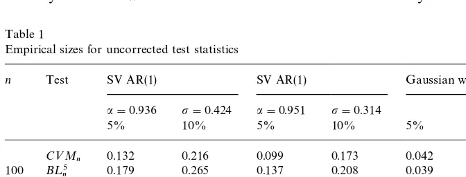
Table 1
Empirical sizes for uncorrected test statistics
n Test SV AR(1) SV AR(1) Gaussian white noise
a"0.936 p"0.424 a"0.951 p"0.314
5% 10% 5% 10% 5% 10%
C<M
n 0.132 0.216 0.099 0.173 0.042 0.081
100 B¸5n 0.179 0.265 0.137 0.208 0.039 0.080
B¸15n 0.148 0.216 0.123 0.186 0.036 0.067
C<M
n 0.288 0.391 0.215 0.313 0.045 0.094
500 B¸5n 0.405 0.500 0.325 0.414 0.053 0.100
B¸15n 0.472 0.586 0.398 0.496 0.047 0.092
(ii) The Box}Ljung}Pierce statistic with K"5. The uncorrected version is denoted byB¸5
n and the corrected version byB¸5n,C.
(iii) The Box}Ljung}Pierce statistic withK"15. The uncorrected version is denoted byB¸15
n and the corrected version byB¸15n,C.
In addition to the conditionally heteroscedastic data, we also studied the performance of these test statistics when the data was actually Gaussian white noise. This is necessary to see how the corrected statistics behave when the data is actually homoscedastic and the correction is unnecessary.
In Table 1, we compare the empirical sizes of the uncorrected versions of the statistics. The sizes were computed by comparingC<M
n,B¸5n andB¸15n with
the asymptotic 5% and 10% critical values of the CrameHr von-Mises, thes25and thes215 distributions, respectively. As is to be expected, the tests based on the uncorrected statistics are oversized when the data is a conditionally hetero-scedastic martingale di!erence. This in#ation in size can be quite severe and is greater for the larger sample size. It is interesting to note that among the three statistics, the CrameHr von-Mises statistic su!ers the least from the problem of size in#ation. When the data are Gaussian white noise and therefore homo-scedastic, all three statistics maintain approximately their nominal size, though
B¸15
n is somewhat undersized when n"100. This might explain why the size
in#ation in B¸15
n is lower than that in B¸5n when n"100 but higher when
n"500.
In Table 2, we compare the sizes of the corrected versions of the statistics. As earlier, the sizes were computed by comparingC<M
n,C, B¸5n,C, andB¸15n,Cwith
the asymptotic 5% and 10% critical values of the CrameHr von-Mises, thes25and thes215 distributions, respectively. As can be seen from the table, the corrected statistics maintain their nominal size even under conditional heteroscedasticity thoughB¸15
n,Cis somewhat undersized whenn"100. Furthermore, it is
Table 2
Empirical sizes for corrected test statistics
n Test SV AR(1) SV AR(1) Gaussian white noise
a"0.936 p"0.424 a"0.951 p"0.314
5% 10% 5% 10% 5% 10%
C<M
n,C 0.036 0.083 0.038 0.087 0.041 0.087
100 B¸5
n,C 0.030 0.065 0.028 0.064 0.048 0.085
B¸15
n,C 0.029 0.062 0.031 0.065 0.041 0.065
C<M
n,C 0.048 0.090 0.057 0.092 0.038 0.094
500 B¸5
n,C 0.049 0.085 0.052 0.086 0.054 0.095
B¸15
n,C 0.056 0.084 0.049 0.092 0.049 0.093
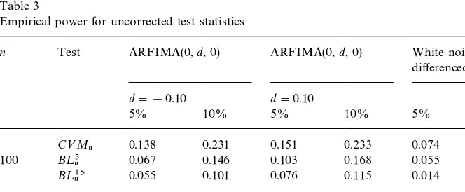
Table 3
Empirical power for uncorrected test statistics
n Test ARFIMA(0,d, 0) ARFIMA(0,d, 0) White noise# di!erenced AR(l) d"!0.10 d"0.10
5% 10% 5% 10% 5% 10%
C<M
n 0.138 0.231 0.151 0.233 0.074 0.120
100 B¸5n 0.067 0.146 0.103 0.168 0.055 0.103
B¸15n 0.055 0.101 0.076 0.115 0.014 0.077
C<M
n 0.578 0.716 0.672 0.773 0.134 0.232
500 B¸5n 0.416 0.571 0.581 0.679 0.132 0.236
B¸15n 0.233 0.367 0.453 0.566 0.105 0.192
In Tables 3 and 4, we compare the empirical power of the uncorrected and corrected versions of the three statistics, respectively. The power calculations were made when the data was generated by the following two alternative models:
(i) A fractionally integrated model (ARFIMA(0,d, 0)) given by (1!B)dX
t"ut, whereMutNare i.i.d. N(0, 1). For the simulations, we chose two
values ofd, !0.1 and 0.1.
(ii) The sum of white noise and the"rst di!erence of a stationary autoregres-sive process of order one. i.e.X
t"vt#>t!>t~1, where>t"0.85>t~1#ut.
The vector (u
t, vt) was chosen to be a sequence of independent bivariate normal
random variables with mean zero and variance covariance matrix given by
diag(p2u, 1). The value of p2u was chosen such that the share of the variance of X
t due to the mean reverting component >t!>t~1, given by
2p2
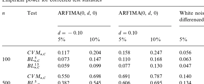
Table 4
Empirical power for corrected test statistics
n Test ARFIMA(0,d, 0) ARFIMA(0,d, 0) White noise# di!erenced AR(l) d"!0.10 d"0.10
5% 10% 5% 10% 5% 10%
C<M
n,C 0.117 0.204 0.158 0.247 0.056 0.117 100 B¸5
n,C 0.073 0.147 0.110 0.168 0.063 0.112
B¸15
n,C 0.059 0.099 0.077 0.130 0.047 0.075
C<M
n,C 0.550 0.698 0.691 0.787 0.140 0.245 500 B¸5
n,C 0.382 0.545 0.606 0.695 0.134 0.250
B¸15
n,C 0.225 0.369 0.451 0.559 0.112 0.207
From Table 4 it is seen that among the three statistics, the corrected CrameHr von-Mises statistic almost always has the highest power against all the three alternatives studied here. The gain in power for the CrameHr von-Mises statistic is the most, however, against the fractionally integrated series, being as high as 17% when the sample size is 500. As discussed earlier, this was to be expected, since, for such models, the individual correlations are small in magnitude even though they decay very slowly to zero. Surprisingly, against the frac-tionally integrated alternative, the Box}Ljung}Pierce statistic at lag 15 has lower power than that at lag 5, even though it uses information from correla-tions upto a greater number of lags. Again, this might be due to the small magnitude of the individual correlations. When the alternative is the sum of white noise and the"rst di!erence of a stationary autoregressive process, both
C<M
n,CandB¸5n,Chave comparable power, which is slightly higher than that of
B¸15
n,C.
By comparing Tables 3 and 4, we also see that the power of the uncorrected and corrected versions of the statistics is virtually the same for the three alternatives considered. Thus, using the corrected statistics does not result in a loss of power when the data is conditionally homoscedastic.
Table 5
Tests for weekly CRSP returns (1962}1985)
C<M
n C<Mn,C
Value-weighted 0.857 0.533
Equal-weighted 11.213 5.988
Asymptotic critical values
5% 0.46
1% 0.74
5. Application to stock prices
In this section, we apply our results to some time series of stock returns. The series that we analyse are weekly #uctuations for two CRSP NYSE-AMEX aggregate porfolios and also monthly returns on the CRSP-NYSE. Both of these data sets were analyzed in Durlauf (1991).
The "rst data sets consists of 1216 weekly returns on value-weighted and equal-weighted CRSP NYSE-AMEX portfolios from September 6, 1962 to December 26, 1985. Following Durlauf (1991), the weekly returns were com-puted using closing Wednesday prices. If the exchange was closed on a Wednes-day, the Thursday price was used and if the exchange was also closed on Thursday, the previous Tuesday price was used. An examination of the sample autocorrelations of the squared returns (not presented here) showed that condi-tional heteroscedasticity is present in both the series. In Table 5 we report values of the C<M test statistic (C<M
n) as well as the corrected C<M statistic
(C<M
n,C) for both these series. As can be seen from the table, we can reject the
null hypothesis of zero correlation at the 1% level of signi"cance for both the series, based upon theC<Mstatistic. The evidence is overwhelming in the case
of the equal weighted returns. However, the correctedC<Mstatistics for both
the series are much smaller. We are no longer able to reject the null hypothesis at the 1% level of signi"cance for the value weighted returns. As a matter of fact, using the tables provided in Anderson and You (1996), one"nds that thep-value for the correctedC<Mstatistic is between 2.5% and 5%. There is still strong
evidence against the null for the equal-weighted returns however.
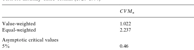
The second data set consisted of 780 monthly returns on the CRSP-NYSE value-weighted and equal-weighted portfolios from January 1926 to December 1990. As before, examination of the sample autocorrelations of the squared returns (not presented here) showed the presence of conditional heteroscedastic-ity in both the series. In Table 6, we report values of theC<Mtest statistic as
well as the corrected C<M statistic for these series. The uncorrected C<M
Table 6
Tests for monthly CRSP returns (1926}1990)
C<M
n C<Mn,C
Value-weighted 1.022 0.348
Equal-weighted 2.237 0.563
Asymptotic critical values
5% 0.46
1% 0.74
smaller and we can no longer reject the null hypothesis at the 5% level for the value-weighted returns. There is some evidence against the null for the equal-weighted returns, though the associatedp-value obtained from Anderson and You (1996) is greater than 2.5%.
6. Conclusions
We have shown that the distribution of the sample spectral distribution function for a white noise series is a!ected by the presence of conditional heteroscedasticity. The asymptotic distribution depends on the covariance structure of the second moments of the series. This causes test statistics based on the sample spectral distribution, such as the CrameHr von-Mises statistic, to have heavily right skewed distributions, which will lead to over-rejection of the martingale hypothesis in favour of mean reversion. This phenomenon is
con-"rmed by Monte Carlo simulations. A non-parametric correction to the test statistics is proposed to account for the conditional heteroscedasticity. The corrected version of the CrameHr von-Mises statistic is shown to have an asymptotic distribution una!ected by conditional heteroscedasticity. A Monte Carlo study of the corrected version of the CrameHr von-Mises statistic shows that the"nite sample distribution behaviour is quite satisfactory for samples as small as a 100 observations. An empirical application to stock returns shows that evidence against the null hypothesis of the random walk can be consider-ably weakened after using the corrected test and accounting for conditional heteroscedasticity.
Acknowledgements
Appendix. (Technical)
Proof of Lemma 1. SinceMh
tNis a Gaussian stationary series with zero mean, it
can be expressed ash
t"+=j/0ajut~j, where+=j/0a2j(RandMutNis a sequence
of independent standard normal variables. Furthermore,Mu
tNandMvtNwill also
be independent. It is trivial to check thatMetNis a martingale di!erence and thus satis"es (i) of Condition A. Furthermore, by using the fact that EMexp(a>)N"
expM0.5a2<ar(>)N for a zero mean Gaussian random variable >, we get
p20,E(e2
t)"p2vexpM2+=j/0a2jN(R, thus verifying condition (ii). Now, by
Lemma 3.5.8 and Theorem 3.5.8 of Stout (1974), z
t,E(e2tDFt~1)"
coupled with the existence of its eighth moment also guarantees (v). By Lemma 3.5.8 and Theorem 3.5.8 of Stout (1974),et~ret~sE(e2
tDFt~1)"et~ret~sztis a
sta-tionary ergodic series for anyr*1,s*1 and hence by Theorem 3.5.7 of Stout (1974), assumption (vi) is also satis"ed. The fact thatMv
tNis an independent zero
mean series with"nite eighth moment and also independent ofMh
tNguarantees
that assumptions (vii) and (viii) are met. Hence, the stochastic volatility model (2) satis"es Condition A.
Proof of Lemma 2. Under the conditions of Lemma 2, it follows by Theorem 2 and the Corollary to Theorem 3 of Nelson (1990), thate
t is a stationary ergodic
martingale di!erence with"nite eighth moments. Thus,Me
tNimmediately satis-"es assumptions (i), (ii), (iv), (v) and (viii) of Condition A. By Theorem 2 of Nelson (1990),p2
t is stationary and ergodic and can be expressed as p2
Hence, by Theorem 3.5.7 of Stout (1974), assumptions (iii) and (vi) of Condition A are also satis"ed. It remains now to show that assumption (vii) of Condition A also holds for this model. For anyq, 2)q)8, consider E(<qi/1esi
ti), where
the s
i are non-negative integers such that at least one si is exactly one and
+is
i)8. We assume without loss of generality thatt1't2'2'tq. Then,
there is some p, 1)p)q, such that s
i"2ji for 1)i(p and sp"2jp#1,
wherej
i are non-negative integers. Thus,
But
tp multiplied by some function of all the othervt. Each such term
has an expectation of zero since the processMv
tNis independent and symmetric
around zero. Furthermore, the conditional expectation of all such terms is still zero by independence. Hence, E[<pi/1esi
tiDFtp~1]"0, which by (A.2) implies
that (vii) of Condition A holds.
Proof of Theorem 3.1. Since ;
n,w()) is location and scale invariant, we will
assume henceforth, without loss of generality, that E(X
t)"0 and<ar(Xt)"1.
Condition (i) holds trivially. We will demonstrate condition (ii) only fork"1 since the argument for generalkfollows by applying the CrameHr}Wold device. To prove condition (ii), we write¹
n,1(t) as
for some integers. From Theorem 2.1 and the fact thatw
n(j)P1 for"xedj, it
Furthermore, though the series MX
tN is not independent, assumption (vii) of
Condition A and the boundedness ofw
n()) allow us to exactly retrace the steps
of Theorem 1 of Grenander and Rosenblatt (1957, p. 188) and conclude that for su$ciently large s, Rsn,1(t) is small in probability uniformly in nand t. More speci"cally, givend'0 andg'0, there exists ansand anN
0such that for all
n'N
assPR. Eqs. (A.5)}(A.8) allow us to apply Proposition 6.3.9 of Brockwell and Davis (1991) and conclude that condition (ii) is satis"ed. To prove condition (iii), we note that
1such that the second term on the right-hand side of (A.9) is less
thang/2 for alln'N
associated with¹sn
only demonstrate the proof forp"2 since the same method applies in the other cases. The result is obtained by verifying the three conditions stated earlier. Condition (i) is again trivially satis"ed. As before, we will prove condition (ii) only fork"1 since the general result follows by applying the CrameHr}Wold device. For some integers, we can writeQ
n(t)"n~1@2XM ~1¹n,2(t) as
Also, assumption (vii) of Condition A implies that E(bK4
j)"O(1). This fact and
the Cauchy}Schwarz inequality imply that E(bK
ibKjbKkbKl)"O(1)"O(n) (A.12)
for anyi, j, k, l. Once again we can retrace the steps in Theorem 1 of Grenander and Rosenblatt (1957, p. 188) and using (A.12) and the boundedness ofw
n())
conclude that (A.7) holds forRsn(t). By using Proposition 6.3.9 of Brockwell and Davis (1991), we conclude thatplim
n?=Qn(t)"0. Finally, condition (iii) can be
shown forQ
n(t) in a manner similar to the one used for¹n,1(t). Thus, we have the
weak convergence ofQ
n(t) (and hence of¹n,2(t)) to zero.
Proof of Theorem 3.3. It is possible (see Anderson and You, 1996) to express
C<M
wheresis sone integer. By assumptions (iii) and (iv) of Condition A, we have
plim
conjunction with assumptions (iv) and (vi) also gives, for "xed j,
plim
n?=(n!j)~1+tn/1~j(Xt!XM )2(Xt`j!XM )2"E(e2te2t`j). Using these results,
it follows from Theorem 2.1 and the fact thatw
n(j)P1 for"xedj, that for"xeds,
assPR. Furthermore, it follows from (12) and the boundedness ofw
n()), that
for some constantM. Hence, lim
s?=
lim
n?=
P(DRsnD'd)"0.
From Proposition 6.3.9 of Brockwell and Davis (1991), we thus get
C<M
Proof of Corollary 3.4. Since the test statistic is location and scale invariant, we will assume throughout this proof, without loss of generality, that E(X
t)"0 and
<ar(X
t)"1. By Lemma 1, the assumptions of Condition A are satis"ed by this
The theorem is proved if sup
1xjxn~Jn
nE(a(2j)(M(R (A.14)
for some constant M, which we show next. To do this, we verify that the conditions of Theorem 5.4.3 of Fuller (1996) hold. We can writena(2
j as
Note that by the Cauchy}Schwarz inequality,f(Z
j,n,>j,n) is a bounded function.
By expanding the product in the numerator of Z
j,n, noting that
E(+lt/1X
t)2"O(l) and applying the Cauchy}Schwarz inequality, it follows that
E(Z2
j,n)"O
A
1
n!j
B
(A.16)for 1)j)n!Jn.
Expanding the squared term in the numerator of >
j,n and letting
is the remainder term. We"rst demonstrate that E(R2
j,n)"O
A
1
By assumption (vii) of Condition A, it follows that both E(+nt/1~jX2
for 1)s)4. These facts together with the Cauchy}Schwarz inequality imply Eq. (A.17). We next show that
E
A
1It can be easily shown that under the assumed model,qj"p4
vexp(4p2h#4cj),
1, where the last inequality follows from the assumption
thataj"O(jj) for some 0(j(1. Using the bound (A.20) in Eq. (A.19) gives us
which in conjunction with (30) proves that E(>
j,n!qj)2"O
A
1
n!j
B
. (A.21)From Eqs. (A.16) and (A.21), it follows that condition (i) of Theorem 5.4.3 of Fuller (1996) is satis"ed with a
qj"p4
vexp(4p2h#4cj), we have 0(C1(infjw1qj)supjw1qj(C2(R for
some constants C
1 and C2. De"ning the set Sj by Sj"Mx, y:DxD)1, Dy!q
jD)C1Nand noting that the functionf(x,y) is a bounded function, we see
that the remaining conditions of Theorem 5.4.3 of Fuller (1996) are satis"ed and thus
Ef(Z
j,n,>j,n)"O
A
1
n!j
B
(A.22)for 1)j)n!Jn. Eq. (A.14) now follows from Eqs. (A.22) and (A.15).
References
Anderson, T.W., 1993. Goodness of "t tests for spectral distributions. Annals of Statistics 21, 830}847.
Anderson, T.W., You, L., 1996. Adequacy of asymptotic theory for goodness-of-"t criteria for spectral distributions. Journal of Time Series Analysis 17, 533}552.
Billingsley, P., 1968. Convergence of Probability Measures. Wiley, New York.
Bougerol, P., Picard, N., 1992. Stationarity of GARCH processes and of some non-negative time series. Journal of Econometrics 52, 115}127.
Brockwell, P.J., Davis, R.A., 1991. Time Series: Theory and Methods, 2nd Edition. Springer, New York.
Cochrane, J.H., 1988. How big is the random walk in GNP? Journal of Political Economy 96, 893}920.
Deo, R.S., 1997. Conditionally heteroscedastic stable processes. Working paper, New York Univer-sity.
de Vries, C.G., 1991. On the relation between GARCH and stable processes. Journal of Econo-metrics 48, 313}324.
Durlauf, S.N., 1991. Spectral based testing of the martingale hypothesis. Journal of Econometrics 50, 355}376.
Fuller, W.A., 1996. Introduction to Statistical Time Series, 2nd Edition. Wiley, New York. Grenander, U., Rosenblatt, M., 1957. Statistical Analysis of stationary Time Series. Chelsea,
New York.
Hannan, E.J., Heyde, C.C., 1972. On limit theorems of quadratic functions of a discrete time series. Annals of Mathematical Statistics 43, 2058}2066.
Nelson, D., 1990. Stationarity and persistence in the GARCH(1, 1) model. Econometric Theory 6, 318}334.
Shephard, N., 1996. Statistical aspects of ARCH and stochastic volatility. In: Cox, D.R., et al. (Ed.), Time Series Models in Econometrics, Finance and Other Fields. Chapman & Hall, London. Stout, W.F., 1974. Almost Sure Convergence. Academic Press, New York.