M P E J
M P E J
M P E J
M P E J
M P E J
M P E J
M P E J
M P E J
M P E J
M P E J
M P E J
M P E J
M P E J
M P E J
M P E J
M P E J
M P E J
M P E J
M P E J
M P E J
M P E J
Mathematical Physics Electronic Journal
ISSN 1086-6655 Volume 13, 2007
Paper 6
Received: Nov 29, 2005, Revised: Dec 6, 2006, Accepted: Oct 14, 2007 Editor: R. de la Llave
Whitney regularity for solutions to the
coboundary equation on Cantor sets
Matthew Nicol
Andrei T¨
or¨
ok
∗Department of Mathematics
University of Houston
Houston, Texas 77204-3008
†Abstract
We prove Whitney regularity results for the solutions of the coboundary equation over dynamically defined Cantor sets satisfying a natural geometric regularity condi-tion, in particular hyperbolic basic sets in dimension two. To do this we prove an analogue of Journ´e’s well-known result in the context of Cantor sets satisfying geomet-ric regularity conditions.
1
Introduction
interested in the situation when Λ might have no interior. Whenever Λ is not open, smoothness is meant in the sense of Whitney.
Results in this direction were first obtained by Livˇsic, for real valued cocycles over Anosov mappings. He showed [6] that if the cocycle g is C1, then the trivialization φ (assumed apriori only measurable) is C1 too. For some linear actions on a torus he also showed [7] that if the cocycle is C∞, respectively Cω, then so is the solution; this was obtained by studying the decay of the Fourier coefficients.
The C∞ (smooth) case was investigated by de la Llave, Marco and Moriy´on [10]. One of the technical results they proved was that if a function is smooth along two transverse foliations which are absolutely continuous and whose Jacobians have some regularity properties, then it is smooth globally. This was proved using properties of elliptic operators. Relying on Taylor expansions, careful error estimates and Morrey-Campanato theory, Journ´e ([4]; see Theorem 1.1 below) proved a similar result without requiring the absolutely continuity of the foliations. Another approach is presented in Hurder and Katok [3], based on an unpublished idea of C. Toll. Here the decay of the Fourier coefficients is used to characterize smoothness. Using the approach in [3], de la Llave proved analogous results in the analytic case [9]. More references are given in [12].
Journ´e’s key result is the following:
Theorem 1.1 [Journ´e [4]] LetFs andFu be two continuous transverse foliations with uniformly smooth leaves of some manifold. If f is uniformly smooth along the leaves of Fs and Fu then f is smooth.
Various modifications have been proven since. We mention in particular work of de la Llave [8, Theorem 5.7], where Whitney regularity was proved, and Vano [19, Lemma 3.2.6]. Our main result is in some sense a technical improvement over de la Llave’s Theorem 5.7: it applies to sets that are less regular (as opposed to de la Llave’s condition (iv)), and that could have measure zero. We state our result in terms of laminations whose leaves satisfy a certain geometric regularity, but we have in mind applications to a class of hyperbolic basic sets.
Recall that if Λ⊂M is an invariant hyperbolic set for a C1 map T, then through each point x ∈ Λ there exists a local stable manifold Wεs(x) and a local unstable manifold Wu
ε(x). We call a hyperbolic invariant set basic if it is locally maximal, that is, Λ = ∩∞
n=−∞Tn(V) for an open set V. A hyperbolic set Λ is basic if and only if it has local product structure: if x, y ∈ Λ are close enough, then the unique point z=Ws
ε(x)∩Wεu(y) belongs to Λ [5, Section 18.4].
Let n ≥ 1, α ∈ (0,1). For an open set U ⊂ Rd, Cn,α(U) consists of functions that are differentiable of order n, have all derivatives bounded, and the n-th partial derivatives are α-H¨older (see [18, Chapter VI]).
and whose union contains the set Λ.
Remark 1.3 Examples of Cn,α-laminations are the stable and unstable foliations of a hyperbolic set for a Cn+1 diffeomorphism.
We describe here the notion of geometric regularity that we are using. Definition 1.4 Fix constants 0< γ <1 andν >0.
(a) A setA contained in aC1-curve Γ is (γ, ν)-homogeneous if for eachx∈A, there is a sequence of points xk∈A converging tox such that distΓ(x, x1)≥ν, and
distΓ(x, xk+1) distΓ(x, xk)
≥γ for k≥1 (1.2) (here distΓ denotes the distance induced on the curve Γ).
(b) A set Λ⊂R2is (γ, ν)-homogeneous with respect to two transverseC1-laminations Ws and Wu if for each p ∈ Λ, the sets Ws(p)∩Λ and Wu(p)∩Λ are (γ, ν)-homogeneous in the corresponding leaves.
Our main result is an extension of Journ´e’s Theorem 1.1.
Theorem 1.5 Let Λ ⊂ R2 be a closed set, and Ws, Wu two transverse uniformly Cn,α-laminations of Λ.
Suppose that φ: Λ → R is uniformly Whitney-Cn,α when restricted to Wεs(x) and Wεu(x) for each x∈Λ. If
• Λ is(γ, ν)-homogeneous with respect to Ws and Wu for some γ, ν >0, and
• Λ has a local product structure: for x, y∈Λ close enough, the (unique) point in the intersection Wεs(x)∩Wεu(y) belongs to Λ,
then φ is Whitney-Cn,α on Λ.
The term “uniformly” above means that the given property holds with uniform con-stants over the whole set Λ.
Remark 1.6 Examples of (γ, ν)-homogeneous sets include hyperbolic basic sets in dimension two (see Proposition 2.2), Anosov systems, and the direct product of one dimensional uniformly homogeneous sets in higher dimensions (see Section 5).
n I
n
L On Rn
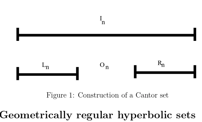
Figure 1: Construction of a Cantor set
2
Geometrically regular hyperbolic sets
We describe a class of dynamically defined two-dimensional Cantor sets to which The-orem 1.5 pertains. First we describe the notion of ‘thickness’ of Cantor sets. This was introduced by Newhouse [11]. A Cantor setK inRis formed by starting with a closed interval and successively removing open intervals of decreasing length. Suppose each open interval On that is removed from a closed interval In leaves behind two closed intervalsLnand Rn (see Figure 1). Let
τn= min{|Ln|,|Rn|} |On| and
σn= |On| max{|Ln|,|Rn|} The quantity
τ(K) = inf n τn
is called the thickness of the Cantor setK. K is called a thick Cantor set if τ(K)>0. We define
σ(K) = inf n σn
and define adistortion-free thick Cantor set to be a thick Cantor setK withσ(K)>0. We say a two dimensional set Λ ⊂ R2 with a lamination is a distortion-free thick Cantor set if for eachp∈Λ,Ws(p)∩Λ andWu(p)∩Λ are distortion-free thick Cantor sets with uniformσ, τ. For more information on thick Cantor sets see [15, Chapter 4, Section 2] and [2].
Lemma 2.1 If Λ is a distortion-free thick Cantor set then Λ is (γ, ν)-homogeneous. Proof: Assume x ∈Λ. To simplify notation, we parametrize Wεs(x) by arc-length, coordinatize so thatx= 0 and assume from now on that points in Λ∩Ws
to zero and satisfying equation (4.1) for some γ. Furthermore γ may be taken as uniform overx∈Λ.
First note that for all n:
(a) στmax{|Ln|,|Rn|} ≤τ|On| ≤min{|Ln|,|Rn|} (b) 1+σ+στστ |In| ≤min{|Ln|,|Rn|}
Suppose x∈In, choosex1 to be the endpoint ofIn furthest fromx. Without loss of generality suppose that x ∈ Ln∩In (exactly the same argument holds if x ∈Rn). Choosex2 to be the endpoint ofLn furthest fromx. Then|x2| ≥ 12|Ln| ≥ 121+σ+στστ |x1| as |x1| ≤ |In|. Taking γ = 2(1+σ+στστ ) we have |x2| ≥ γ|x1|. Repeat this procedure, taking Ln to be In and noting that x2 is the endpoint of Ln furthest from x. The argument for the unstable foliation is the same.
Proposition 2.2 Two-dimensional hyperbolic basic sets are (γ, ν)-homogeneous. Proof: This follows from [15, Chapter 4, Section 1] and Lemma 2.1. Note that both local stable and local unstable manifolds are dynamically defined Cantor sets for an expanding map (an expanding map in backwards time for stable manifolds). By the uniform bounded distortion estimates on such maps [15, Chapter 4, Section 1] σn,τn are uniformly bounded away from zero.
3
Livˇsic regularity results
The regularity results for the Livsic equation (1.1) state that under certain conditions a measurable solution is actually H¨older, or that a continuous solution is actually (Whitney) smooth.
Suppose that Λ is a hyperbolic basic set and µis an ergodic Gibbs measure corre-sponding to a H¨older continuous potential.
We first show that if we have a measurable coboundary φfor a H¨older real-valued cocyclegthenφhas a H¨older version, that is, there exists a H¨olderφ′ such thatφ′ =φ, µa.e. This result is not new and the main idea is due to Livsic [7] (for related results see [1, 13, 14, 16, 17]). We sketch its proof only for completeness.
Proposition 3.1 Let Λ ⊂ U ⊂ M be a hyperbolic set for the C1 embedding T : U → M. Suppose that Λ is equipped with an ergodic Gibbs measure µ. Assume that g :U → R is η-H¨older, η > 0, and there is a µ-measurable function φ: Λ→ R such that
Proof: For x ∈Λ define gN(x) :=g(TN−1x) +· · ·g(T x) +g(x). If y ∈Wεs(x) then |gN(x)−gN(y)| ≤PNi=0−1|g(Tix)−g(Tiy)| ≤C1(PN−1i=0 ληi)d(x, y)η for some 0< λ <1.
Thus for all N ≥0 and y∈Ws ε(x)
|φ(x)−φ(y)| ≤C2d(x, y)η+|φ(TNx)−φ(TNy)|
By Lusin’s theorem there exists a set Λ′ ⊂Λ such that µ(Λ′)> 12 and φrestricted to Λ′ is uniformly continuous. SinceT is ergodic with respect to µ, for µa.e. x∈Λ,
lim N→∞
1
N#{i|0≤i≤N−1, T
i(x)∈Λ′}=µ(Λ′)> 1
2 (3.2) The ergodic Gibbs measure µ is a product measure, that is, for µ a.e. x ∈ Λ, on a neighborhood of x, the measure µ is equivalent to µsx ×µux, where µsx and µux are the conditional measures ofµ along the stable Wεs(x) and unstable Wεu(x) leaves respectively. Sinceµis locally a product measure,µa.e. x∈Λ has the property that for µs
x a.e. y∈Wεs(x) equation (3.2) holds. Hence forµa.e. x∈Λ, forµsx a.e. y∈Wεs(x) we may choose a subsequenceNi so that|φ(TNix)−φ(TNiy)| →0. Thusµa.e. x∈Λ has the property that for µsx a.e. y ∈ Wεs(x), |φ(x) −φ(y)| ≤ C2d(x, y)η. Similar considerations show that µ a.e. x ∈ Λ has the property that forµu
x a.e. y ∈ Wεu(x), |φ(x)−φ(y)| ≤ C3d(x, y)η. The local product structure for µ implies that φ has an η-H¨older version (see [5, Proposition 19.1.1]).
Next, we show that the regularity can be improved from C0 to Cn,α for hyperbolic basic sets in dimension two:
Theorem 3.2 Let M be a two-dimensional manifold, and Λ ⊂U ⊂ M a hyperbolic basic set for theCn,α embedding T :U →M. Assume that for g∈Cn,α(U), there is a continuous function φ: Λ→R such that
(φ◦T−φ)(x) =g(x), x∈Λ. (3.3) Then φ is Cn,α in the Whitney sense, that is, it admits a Cn,α extension to a neighborhood of Λ.
The proof of this theorem follows the “classic” approach [7, 10, 4]: first show thatφ is regular along the stable and unstable foliations, and then prove that such a function is regular globally. The first step is straightforward, and presented in Lemma 3.3. The second part, in view of Proposition 2.2, is Theorem 1.5.
Lemma 3.3 Let M be a manifold, andΛ⊂U ⊂M a hyperbolic basic set for the Cn,α embedding T :U → M. Assume that for g ∈Cn,α(U), there is a continuous function φ: Λ→R such that
Proof: We extend φ through the cohomology equation (3.4). Using the notation F|b
a=F(b)−F(a), we obtain
φ(y)−φ(x) =− N X n=0
g◦Tn|yx+φ◦TN+1|yx Therefore, define
e
φs(y) :=φ(x)− ∞ X n=0
g◦Tn|yx, y∈Wεs(x), e
φu(z) :=φ(x) + ∞ X n=1
g◦T−n|zx, z∈Wεu(x), The series converge uniformly in Cn,α(Ws
ε(x)), respectively Cn,α(Wεu(x)). Therefore, e
φs and φeu are inCn,α, and vary continuously with the leaf.
Assume x, y ∈Λ and t ∈Wεs(x)∩Wεu(y). By the local product structure, t ∈Λ. Therefore, by (3.4) and the continuity of φ,
e
φs(t) =φ(x)− ∞ X n=0
[φ◦T−φ]◦Tn|tx =φ(x)−h−φ|tx+ lim n→∞φ◦T
n|t x i
=φ(t). Similarly, usingT−1instead ofT, we obtain thatφeu(t) =φ(t). Thus, the two extensions coincide over Wεs(Λ)∩Wεu(Λ).
As an immediate corollary of Proposition 3.1 and Theorem 3.2,
Corollary 3.4 Let M be a two-dimensional manifold, and Λ⊂ U ⊂M a hyperbolic basic set for theCn,α embedding T :U →M. Assume that for g∈Cn,α(U), there is a measurable function φ: Λ→R such that
(φ◦T−φ)(x) =g(x), x∈Λ. (3.5) Then φ is Cn,α in the Whitney sense, that is, it admits a Cn,α extension to a neighborhood of Λ.
4
Journ´
e revisited
We prove Theorem 1.5 in this section. The proof follows the method of Journ´e [4], with a few adjustments.
Our proof similarly uses approximating polynomials but we will use [18, §VI.2.3, Theorem 4] which gives sufficient conditions under which a function extends in the Whitney sense from a closed set.
Given our homogeneity assumption, we can select on each leaf a grid whose spacing is close to being a geometric progression (that is, points are at distances approxima-tively {ωk} from the origin). The local product structure yields a two-dimensional grid, on which we interpolate the functionφ by a sequence of polynomials. We prove that the lower-order coefficients of these polynomials converge, thus yielding a local approximation Q(q;p) toφ(q) (indexed by each pointp of the set Λ). These approxi-mating polynomials ‘correspond’ to the Taylor polynomials of φ. We then show that these local approximations satisfy the hypothesis of the Whitney Extension Theorem stated in [18, §VI.2.3, Theorem 4]. The homogeneity plays an important role here as well.
Notation 4.1 Unless stated otherwise, all constants are uniform onΛ. In particular, we will use the letter C for various constants of this type, even if their values are different. For simplicity of exposition we will refer to Ws
ε(x) as local stable manifolds and to Wεu(x) as local unstable manifolds.
Given nearby points x, y∈Λ, we denote [x, y] := Wεs(x)∩Wεu(y).
(a)
Regular grid from homogeneity
We show that the homogeneity assumption provides a quite regular “grid”. Lemma 4.2 Suppose {rk} is a sequence of numbers converging to zero such that
|rk+1|
|rk| ≥γ for k≥1 (4.1) for some γ >0. Let ω∈(0, γ) and definek0 := [logω(|r1|)]. Define R={|rk|}. Then the intersection R ∩[ωk+1, ωk]is nonempty for each k≥k
0.
In particular, there is a decreasing subsequence in R, which we denote also by |rk|, such that|rk| ∈[ω2k+1, ω2k] for 2k≥k0.
Proof: Notice first that we may assume that the sequence |rk|is strictly decreasing. Indeed, if |rℓ+1| ≥ |rℓ|, then property (4.1) is preserved after dropping the term|rℓ+1| from the sequence and relabeling the remaining terms.
(b)
Approximation by polynomials
The goal of this subsection is the following local approximation result:
Theorem 4.3 Under the assumptions of Theorem 1.5, there are constants ε′, C′ >0 and for each p∈Λ a polynomial Q(·;p) of degree n, such that
|φ(q)−Q(q;p)| ≤C′|q−p|n+α for q ∈Λ, |q−p|< ε′. (4.2) Most arguments are adapted from [4].
Let p ∈Λ. Since the consideration is local we make a Cn,α change of variables so that the local stable and unstable manifolds passing throughp become the coordinate axes through the origin. The theorem is a consequence of the following Lemma, which we prove later.
Lemma 4.4 Given κ >0 large enough and the cone K ={(u, v) ∈R2 : |v| ≤κ|u|}, there is a polynomial Q = QK of degree n and constants C1 = C1(κ), ε1 = ε1(κ) > 0 such that
|φ(z)−Q(z)| ≤C1|z|n+α for z∈Λ∩ K ∩Bε1, where Br denotes the ball of radius r centered at the origin.
The constants C1 andε1 are uniform with respect to p∈Λ. Assuming the above Lemma, we prove next Theorem 4.3. Proof of Theorem 4.3
Using Lemma 4.4, we can also construct a polynomial Q′ approximating φon the coneK′
={(u, v) ∈R2 : |u| ≤κ|v|}centered on the unstable manifold. By choosing κ large enough, we can achieve thatV = Λ∩ K ∩ K′ ∩Bε1 is not Zariski closed (indeed, the homogeneity assumption implies that the origin is an accumulation point of both Λ∩Wεs(0,0) and Λ∩Wεu(0,0), and the product structure gives a two-dimensional “grid” inV).
This implies that the n-th degree polynomials Q and Q′ have to coincide, because they have a contact of order higher thann onV.
This establishes that at the point p, in the coordinates used to linearize its stable and unstable manifolds,Qis a local approximation of φof order n+α.
Note that the relevant constants of Lemma 4.4, ε1 and C1, are uniform in p ∈Λ, hence so will the constants ε′ and C′ of Theorem 4.3.
The remainder of the section is devoted to the proof of Lemma 4.4. This proof is divided into a few subsections. By our reduction so far, p is the origin inR2 and the coordinate axes are leaves of the two laminations.
Interpolating polynomials
We will use the following interpolation result of Journ´e, with corresponding constants from Lemma 1 of Journ´e denoted by the subscriptJ.
Lemma 4.5 (Journ´e [4], Lemma 1) Fix n ≥ 1. For each B ≥ 1, there are ε = εJ(B)>0 and C =CJ(B)>0 with the following property: if the collections of points {zk,ℓ : 0 ≤k ≤n,0≤ ℓ≤n} ⊂ R2, {xk : 0≤ k≤ n} ⊂ R, {yℓ : 0≤ ℓ≤n} ⊂ R satisfy
R/η < B and |zk,ℓ−(xk, yℓ)| ≤εη where R = sup
k,ℓ
|zk,ℓ|, η = inf
(k,ℓ)6=(k′,ℓ′)|zk,ℓ−zk ′,ℓ′|,
then for any values{bk,ℓ : 0≤k≤n,0≤ℓ≤n} ⊂R, there exists a unique polynomial p(x, y) = X
0≤p,q≤n
cpqxpyq such thatp(zk,ℓ) =bk,ℓ. Moreover,
X p,q
|cpq|Rp+q≤Csup k,ℓ
|bk,ℓ|. (4.3) Since φ(·,0) and φ(0,·) are Cn,α (and therefore Lemma 4.4 holds for them by approximating with the Taylor polynomial), we can replaceφ(x, y) byφ(x, y)−φ(x,0)− φ(0, y) +φ(0,0). Thus, we may assume thatφvanishes along the axes.
We begin by selecting a convenient grid on each axis. Along the x-axis (which we assume to be the stable direction) we take a sequence of points (r′
k,0) ∈Λ, k≥0, converging to (0,0) and satisfying the homogeneity condition (4.1). We take a sequence (0, s′k)∈Λ along the unstable direction (which we assume to be the y-axis) satisfying bounds similar to (4.1).
By Lemma 4.2, passing to a subsequence, we may assume that the two sequences are similarly spaced: |rk′|,|s′k| ∈[ω2k+1, ω2k] fork≥k0, whereωandk0 are determined using Lemma 4.2 for the two sequences involved. Moreover, by our (γ, ν)-homogeneity assumption, we can arrange thatω=γ/2, and|r′
1|,|s′1|are of orderε1, uniformly with respect to p∈Λ, where ε1 >0 will be determined later.
Notation 4.6 Assume given sequences (r′k,0),(0, sk′) ∈Λ as above, and let w ∈ Λ∩ K ∩Bε1. Consider the points (xw,0) = [p, w]∈Λ, (0, yw) = [w, p]∈Λ.
We construct a new sequence of points (rk,0) ∈Wεs(p)∩Λthat includes(xw,0)and still has a regular spacing. We proceed as follows: if |r′
m+2|<|r′m+1|<|xw| ≤ |r′m|< |r′m−1|, then we drop r′m+1 and r′m, and define rm+1 =xw, rk=r′k for k≥m+ 2and rk =rk−1′ for k ≤m. Thus, the x-coordinates of the new sequence in Wεs(p)∩Λ are · · ·, rm+3 =r′m+3, rm+2 =r′m+2, rm+1=xw, rm=rm−1′ , rm−1 =rm−2′ ,· · ·.
We proceed similarly with the points (0, s′ℓ)∈Wεu(p)∩Λ to incorporate (0, yw). For k, ℓ large enough, use the local product structure to define zk,ℓ := [(0, sℓ),(rk,0)] =Wεu((rk,0))∩Wεs((0, sℓ))∈Λ.
The continuity inC1 of the stable and unstable leaves implies that |[(x,0),(0, y)]−(x, y)|=o(|(x, y)|).
Introduce the “rectangular” grid Sk,ℓ = {(0,0)} ∪ {(rk′,0) : k ≤ k′ < k+n} ∪
{(0, sℓ′) :ℓ≤ℓ′ < ℓ+n} ∪ {(zk,ℓ) :k≤k′ ≤k+n, ℓ≤ℓ′ ≤ℓ+n}.
For each kandℓ, denoteηk,ℓ:= inf{|z−z′| : z, z′ ∈Sk,ℓ, z6=z′},Rk,ℓ:= sup{|z| : z∈Sk,ℓ}, and Tk:= max{|rk|,|sk|}.
Then there are constants C0,k1, independent of z, such that fork, ℓ≥k1 : • Rk,ℓηk,ℓ < C0 as long as|k−ℓ| ≤1.
• |zk,ℓ−(rk, sℓ)| ≤ εJ(C0C0 )|(rk, sℓ)|for|k−ℓ| ≤n. • C01 ω2k ≤T
k ≤C0ω2k.
whereεJ(C0) is the corresponding constant from Lemma 4.5.
Remark 4.7 The points z to which Lemma 4.4 applies are those corresponding to rk, sℓwithk, ℓ≥k1, henceε1=O(ωk1). During the proof we might have to decreaseε1, which means thatk1 will increase accordingly. Note however that the three properties listed above remain valid after such a change.
In light of Lemma 4.5 we conclude that fork≥k1 there exists a unique polynomial P(x, y) = X
0≤p,q≤n
cpqxpyq which interpolates φon each gridS of formSk,k i.e.
P(z) =φ(z) forz∈S.
Furthermore X p,q
|cpq|Rp+qS ≤Csup{|φ(z)| : z∈S} (4.4) where C=CJ(C0) is given by Lemma 4.5, the supremum is taken over the grid used for the interpolating polynomial, andRS is Rk,k.
Consecutive interpolations
Take k ≥ k1 and let P and P′, denote respectively the polynomials of degree n in x andy which interpolateφon Sk,k, respectively Sk,k+1. We denote their coefficients by cpq, respectively c
Instead, we prove in this subsection relation (4.10), which implies the intermediate result (see relation (4.11) below)
But on these points, by construction,P′(z
k′,k+n) =φ(zk′,k+n). So in fact we need only
estimate|φ(zk′,k+n)−P(zk′,k+n)|fork≤k′≤k+n.
For k′ as above, parametrizeWu
ε(rk′,0) by they coordinate. We denote a point on
Wu
ε(rk′,0) by zk′(y) = (xk′(y), y).
Consider the interval Ik := [−C2Tk, C2Tk], where the constantC2, independent of k, is chosen so that the region of the unstable leaf parametrized byIk contains all the points in (Wu
ε(rk′,0)∩Sk,k)∩ K for all k≥k1 and k≤k′ < k+n.
By the hypothesis, there is a uniformly-Cn,α extension of φ to the local unstable leaves of Λ. We refer to this extension whenever we evaluateφ outside the set Λ. We will show that |φ(zk′(y))−P(zk′(y))|=O(Tkn+α) for k≤k′ ≤k+n and y∈Ik.
Fixk′ betweenkandk+n. To simplify the notation, denote by a tilde the functions evaluated on Wεu(zk′) via its parametrizationy7→zk′(y). That is,fe(y) =f(zk′(y)). If
not explicitly stated, these functions have domainIk.
We collect the necessary estimates in the following lemma:
(iii) If p+q≤nthen has at least one zero, denoted bytj, in this interval. Hence,
|d
norm of such a term can be bound by kDxpk′′y We will not write explicitly the uniform bound over the set Λ of theCn,α-norm of xk′
(this is determined by the uniform lamination Wu).1 Note that |x
k′(0)| ≤ Tk, hence
These estimates prove that the first term in the right-hand side of (4.7) is bounded by CTkp+q−n−α kxk′kCn,α(Ik), as desired. If D is not a constant then kDkC0 ≤
1
Ckxk′kCn(Ik), and we obtain the desired bound for the other two terms in the right-hand side of (4.7). If D is a constant, then we must have had q =n, q′ = 0, p =p′, hence the H¨older norm in the third term of (4.7) is zero, and the second term satisfies the desired bound (in this case the first term vanished as well).
The relation (iii) is proven similarly.
Relation (iv) is an immediate consequence of the estimates (ii) and (iii).
Next, we bound the kxk′kCn,α(Ik) term by choosing ε1 >0 sufficiently small. Since the local (un)stable manifolds are continuous in theCn,αtopology and the leaf through the origin coincides with the vertical axis, givenδ >0, we may chooseε1>0 sufficiently small so that
kxk′kCn,α(Ik)< δ (4.8) whenever |rk′|< ε1 and y∈Ik.2
Given our choice of the sequence of pointsrkandsℓ, we may increasek1so that (4.8) holds for allk≥k1 (recall thatrk1 is at distance approximatelyω2k1 from the origin).
Since, by hypothesis, φ∈Cn,α(Wu
ε(rk′,0)) uniformly3, we have
k d n
dynφ(y)kαe ≤C. (4.9) From (4.5), (4.9), (4.6) we obtain that
|(φ−P)(zk′(y))| ≤CTkn+α+Cδ
X p+q>n
|cp,q|Tkp+q+C X p+q≤n
|cp,q|Tkn+α (4.10) fory∈Ik.
By evaluating the above relation at zk′,k+n (recall that P′(zk′,k+n) = φ(zk′,k+n)),
and using (4.3) forP−P′ on Sk,k+1, we obtain that X
p,q
|c′p,q−cp,q|Tkp+q≤C(Tkn+α+δ X p+q>n
|cp,q|Tkp+q+ X p+q≤n
|cp,q|Tkn+α). (4.11)
Convergence of interpolating polynomials
We let P2k denote the interpolation polynomial corresponding to the grid Sk,k, and P2k+1 denote the interpolation polynomial corresponding to the grid Sk,k+1. Equa-tion (4.11) relates the coefficients of P2k+1 to P2k and the same line of reasoning relates the coefficients ofP2k+2 toP2k+1 except that we use the smoothness ofφalong the other lamination. Recall (see the properties of the grid listed on page 11) that Tk = max{rk, sk} is comparable to ω2k. We will be sloppy with notation and letTj/2 denote T[j/2].
Denote by cmpq the coefficient of xpyq inPm.
2
Here the transverseCn,α-continuity of the lamination is used. 3
We will show that, by reducingε1, there areK, m0 large enough, such that We proceed by induction. We first determine when (4.12) for m implies (4.12) for m+1. We claim that this implication (which is a consequence of equation (4.14) below) holds for all K ≥ K∗, m0 ≥ m∗0, δ ≤ δ∗, where the ∗-ed values depend only on the constant C that appears in equation (4.11). We saw thatδ can be made as small as desired by reducing ε1. Next, we pick m0 ≥ max{m∗0, k1} (recall that k1 depends on ε1). Finally, we can further increaseK in order to satisfy (4.12) for m=m0+ 1, the initial step of the induction.
We now justify our claim. From equation (4.11) and the bound KPm−1j=m0(Tj/2)n+α−p−q for |cmpq| given by the induction assumption, relation (4.12) will hold form+ 1 provided
C Note that, by (4.11), (4.14) implies (4.13) as well.
The first term in (4.14) is less than (1/3)KTm/2n+α if K is chosen large enough. Consider the second term divided by the right-hand side,KTm/2n+α:
CKδ
is CKTm/2n+αPp+q≤nTm0n+α−p−q/2 , therefore, taking m0 sufficiently large, we may ensure that this term is less than (1/3)KTm/2n+α as well.
This proves our claim about the values of K, m0 and δ for which equation (4.14) holds, and therefore completes the proof of relations (4.12) and (4.13).
End of proof of Lemma 4.4
By now the constants K, m0, are determined, and uniform on Λ. Reduce once more ε1 so that k1 ≥m0 (recall thatε1 =O(ωk1)).
We describe the coefficients ℓpq of the polynomial Q of degree n mentioned in Lemma 4.4. Recall that Pm(x, y) = Pp,qcmpqxpyq. If p+q > n then we set ℓpq = 0 whereas if p+q≤nthen we define
ℓpq = lim m→∞c
m pq. The limit exists by (4.13).
We claim that, for any C(1) >0, there isC(2) >0, such that for allm≥m0, |Q−Pm| ≤C(2)Tm/2n+α (4.15) provided|x|,|y| ≤C(1)Tm/2.
By (4.12), if p+q > nthen|cm
pqTm/2p+q|=O(Tm/2n+α). Ifp+q≤n, by (4.13) we obtain that
|cmp,q−cm+kp,q | ≤K m+k−1X
j=m
Tj/2n+α−p−q and hence letting k→ ∞
|(cmp,q−ℓp,q)Tm/2p+q| ≤KTm/2n+α ∞ X j=0 ¡
T(m+j)/2/Tm/2
¢n+α−p−q ≤CKTm/2n+α
∞ X j=0
(ωj)n+α−p−q which isO(Tm/2n+α). These estimates imply the validity of equation (4.15).
In addition to the bound obtained above for |cmpqTm/2p+q|, p+q > n, from (4.12) one also obtains upper bounds for |cm
pq|, p+q ≤n. Note that all these hold uniformly on Λ for m≥m0. Using these, relation (4.10) implies that
|(φ−Pm)(zk′(y))| ≤C(3)Tn+α
By the triangle inequality, (4.15) and (4.16) imply |(Q−φ)(zk′(y))| ≤C(4)Tn+α
m/2 if |y| ≤C2Tm/2. Thus, we obtain that
|Q(w)−φ(w)| ≤C1|w|n+α for w∈ K ∩(∪k≥m0Wεu(rk,0)).
In order to finish the proof, notice that by the relabeling introduced in Notation 4.6, we can include any pointw∈ K ∩Λ∩Bε1 in the above union. Forw, w′ ∈ K ∩Λ∩Bε1, we obtain two pairs of sequences {rk, sk}k≥m0 on the stable, respectively unstable, manifold of the origin. But these sequences differ only at finitely many positions. Therefore, the limit polynomial Qdoes not depend on the pointw.
(c)
Whitney regularity
We prove here the following:Theorem 4.9 The conclusion of Theorem 4.3 and our homogeneity assumptions on the set Λ imply that φ isCn,α(Λ) in the Whitney sense.
We will show that functions φ(ℓ), derived from the approximating polynomials Q(q;p) defined on the closed set Λ satisfy conditions (16) and (17) of [18, §VI.2.3] and hence by [18,§VI.2.3, Theorem 4]φadmits a Whitney extension toR2.
According to [18, §VI.2.3, Theorem 4], the conclusion of Theorem 4.9 follows from Lemma 4.10 below. We begin by introducing more notation, relying on the polynomials Q(q;p) constructed in Theorem 4.3.
Define φ(ℓ): Λ→Rby
Q(q;p) = X |ℓ|≤n
φ(ℓ)(p)(q−p) ℓ ℓ! ,
where ℓ = (ℓ1, ℓ2, . . . , ℓd) is a multi-index, ℓ! = ℓ1!. . . ℓd!, |ℓ| = ℓ1 +· · · +ℓd and xℓ =xℓ11 . . . xℓdd forx= (x1, . . . , xd). Here d= 2. Note that φ0 =φ.
For a multi-index j with|j| ≤n, define the polynomials Qj(q, p) :=
X |ℓ+j|≤n
φ(ℓ+j)(p)(q−p) ℓ ℓ! .
Note thatQ0(q;p) =Q(q;p). LetRj(q;p) =φ(j)(q)−Qj(q;p) for |j| ≤n. Lemma 4.10 Under the assumptions of Theorem 4.9,
Proof: Note that the case |j|= 0 is exactly the conclusion of Theorem 4.3. By [18, Lemma VI.2.3.1], if a, b∈Λ, then
Q(x;b)−Q(x;a) = X |j|≤n
Rj(b;a)
(x−b)j j! .
For x∈ Λ thenQ(x;b)−Q(x;a) = [φ(x)−R0(x;b)]−[φ(x)−R0(x;a)] =R0(x;a)− R0(x;b), and we obtain
X 0<|j|≤n
Rj(b;a)
(x−b)j
j! =Fa,b(x), (4.17) whereFa,b: Λ→R,Fa,b(x) :=R0(x;a)−R0(x;b)−R0(b;a). That is, the valuesRj(b;a) are the coefficients of a polynomial of degreeninterpolating the functionFa,b: Λ→R. Such a polynomial is uniquely determined if relation (4.17) holds at (n+ 1)2 points x ∈ Λ spaced as in Lemma 4.5 of Journ´e, and relation (4.3) of that lemma gives the desired upper bound. We describe next the details.
Fix a, b ∈ Λ. By our assumptions on Λ, there are points xi ∈ Wεs(a)∩Λ, yi ∈ Wεu(a)∩Λ, 0≤i≤n, such that
|a−b|/C ≤min
i6=j |xi−xj| |a−b|/C≤mini6=j |yi−yj| max|xi−a| ≤ |a−b|/2 max|yi−a| ≤ |a−b|/2.
Consider the grid (centered at b) determined by zi,j =Wεu(xi)∩Wεs(yj) ∈ Λ. Then max{|a−zi,j|,|b−zi,j|} ≤C|a−b|, and there is a uniform (with respect to|a−b|) bound on the “R/η” of Journ´e (because bothR and η are of order |a−b|). By Theorem 4.3, the former property also implies that |Fa,b(zi,j)| ≤ C|b−a|n+α. Lemma 4.5 can be applied to this interpolating grid. Inequality (4.3) becomes
X 0<|j|≤n
|Rj(b;a)||a−b||j|≤C|a−b|n+α, which gives the desired conclusion.
5
Sets in higher dimensions
Most of our discussion has concerned dimension two, where the homogeneity condition is automatically satisfied for hyperbolic basic sets. It is possible to give geometric conditions on sets in dimensionsd≥3 for the analog of our results to hold: for example a set inRd which is the direct product of done-dimensional (γ, ν) homogeneous sets.
References
[1] M. J. Field and W. Parry: Stable ergodicity of skew extensions by compact Lie groups, Topology,38(1) (1999), 167–187.
[2] B. Hunt, I. Kan and J. Yorke: When Cantor sets intersect thickly, Transactions AMS. 339, No. 2(1993), 869–888.
[3] S. Hurder and A. Katok: Differentiability, rigidity and Godbillon–Vey classes for Anosov flows, Publ. Math. Inst. Hautes Etudes Sci. 72(1990), 5–61.
[4] J.-L. Journ´e: A regularity lemma for functions of several variables,Revista Matem-atica Iberoamericana 4(1988), 187–193.
[5] A. Katok and B. Hasselblatt: Introduction to the Modern Theory of Dynami-cal Systems (Encyclopedia of Mathematics and its Applications, 54, Cambridge University Press, 1995.)
[6] A. N. Livˇsic: Homology properties of U systems,Math. Notes 10(1971), 758–763. [7] A. N. Livˇsic: Cohomology of dynamical systems,Math. USSR Izvestija6 (1972),
1278–1301.
[8] R. de la Llave: Smooth conjugacy and S-R-B measures for uniformly and non-uniformly hyperbolic systems, Commun. Math. Phys. 150 (2), (1992), 289–320. [9] R. de la Llave: Analytic regularity of solutions of Livsic’s cohomology equations
and some applications to analytic conjugacy of hyperbolic dynamical systems,Erg. Th. Dyn. Syst.17(1997), 649–662.
[10] R. de la Llave, J. M. Marco and R. Moryi´on: Canonical perturbation theory of Anosov systems and regularity results for Livsic cohomology equation,Annals of Math.123 (1986), 537–612.
[11] S. Newhouse: Nondensity of Axiom A(a) on S2,Proc. Sympos. Pure. Math. 14, Amer. Math. Soc., Providence, R. I. , 1970, 191–202.
[12] V. Nit¸ic˘a and A. T¨or¨ok: Regularity of the transfer map for cohomologous cocycles, Erg. Th. Dyn. Syst. 18(1998), 1187–1209.
[13] M. Nicol and M. Pollicott: Measurable cocycle rigidity for some non-compact groups, Bull. LMS31, (1999) 592–600.
[14] M. Nicol and M. Pollicott: Livsic’s Theorems for Semisimple Lie Groups,Erg. Th. Dyn. Syst.21 (2001) 1501–1509.
[15] J. Palis and F. Takens: Hyperbolicity and sensitive chaotic dynamics at homoclinic bifurcations, CUP, 1993.
[16] W. Parry and M. Pollicott: The Livsic cocyle equation for compact Lie group extensions of hyperbolic systems, J. London Math. Soc.(2) 56(1997), 405–416. [17] M. Pollicott and C. Walkden: Livˇsic theorems for connected lie groups, Trans.
[18] E. Stein: Singular Integrals and Differentiability Properties of Functions. Prince-ton University Press, New Jersey 1970.