Full Terms & Conditions of access and use can be found at
http://www.tandfonline.com/action/journalInformation?journalCode=ubes20
Download by: [Universitas Maritim Raja Ali Haji] Date: 12 January 2016, At: 23:12
Journal of Business & Economic Statistics
ISSN: 0735-0015 (Print) 1537-2707 (Online) Journal homepage: http://www.tandfonline.com/loi/ubes20
Moment-Based Copula Tests for Financial Returns
Yi-Ting Chen
To cite this article: Yi-Ting Chen (2007) Moment-Based Copula Tests for Financial Returns, Journal of Business & Economic Statistics, 25:4, 377-397, DOI: 10.1198/073500107000000115
To link to this article: http://dx.doi.org/10.1198/073500107000000115
Published online: 01 Jan 2012.
Submit your article to this journal
Article views: 119
View related articles
Moment-Based Copula Tests for
Financial Returns
Yi-Ting CHEN
Institute of Economics, Academia Sinica, Taipei 115, Taiwan (ytchen@gate.sinica.edu.tw)
We propose a class of moment-based tests for copulas in a parametric multivariate dynamic context for financial returns. The proposed method takes into account the effect of estimation uncertainty. This effect is quite important but often is ignored in related studies. Our method can be applied to generate various tests to detect copula misspecification in different directions. In particular, on the basis of the conditional probabilities of quantile exceedances (Kendall’s tau), it generates the tail-dependence tests (the concor-dance test) that can be used to investigate whether the copula being tested is suitable for characterizing the true tail dependence (concordance) structure. Such tests may be useful for exploring the cross-dependence structures of financial returns that are essential for risk management and other purposes. The Monte Carlo simulation supports the validity of our method. As a demonstrative application, we also apply these tests to an empirical study of stock market relationships.
KEY WORDS: Copula; Cross-dependence; Method of moments; Specification test.
1. INTRODUCTION
There is a rapidly growing interest in modeling the cross-dependence structures of financial returns by methods involv-ing copulas that deal with different problems, such as market relationships, value at risk (VaR), derivatives pricing, portfo-lio optimization, and financial contagion (see, e.g., Cherubini, Luciano, and Vecchiato 2004). The rising popularity of this approach may be explained by its flexibility in accommodat-ing different return distributions and various cross-dependence structures. This flexibility permits researchers to be free of the classical scope of normality and linear correlation (see, e.g., Embrechts, Lindskog, and McNeil 2003 for its importance in financial economics). Nevertheless, there is a wide variety of parametric copulas that could imply quite different cross-dependence structures (see, e.g., Hutchinson and Lai 1990; Joe 1997). To avoid the biased conclusions caused by copula mis-specification, we should check the adequacy of copula models in characterizing the true cross-dependence structures by for-mal statistical tests.
In empirical studies, researchers are used to choosing copu-las based on the Akaike information criterion or other similar criteria. Another popular approach is to evaluate copulas based on Rosenblatt’s (1952) multivariate probability integral trans-formation (PIT) theorem. This approach is closely related to the issue of evaluating the (multivariate) conditional probability density models, studied by Diebold, Gunther, and Tay (1998) and Diebold, Hahn, and Tay (1999), among others. The PIT the-orem implies that the derivatives of the true copula, taken with respect to its margins and evaluated at the true PIT of returns, must be U(0,1) distributed. Accordingly, several studies ap-ply the classical goodness-of-fit tests, such as the Kolmogorov– Smirnov test or Pearson’s chi-squared test, to check this uni-formity hypothesis or its variants (see, e.g., Klugman and Parsa 1999; Breymann, Dias, and Embrechts 2003). However, these classical tests are designed for the simple hypotheses that con-tain no unknown parameters, and their practical applications may not be theoretically valid for the reasons described later.
It is well recognized that financial returns have the stylized fact of volatility clustering, and stock returns may even have the leverage effect (see, e.g., Engle 1982; Bollerslev 1986; Nel-son 1991). This means that financial returns are unlikely to be
dynamically independent. As such, the role of returns in the PIT should be replaced with the standardized residuals of cer-tain properly specified generalized autoregressive conditional heteroscedasticity (GARCH)-type models that characterize the dynamic dependence structures. The parametric copula-based multivariate dynamic (CMD) models introduced by Hu (2006), Jondeau and Rockinger (2006), and Patton (2006a,b) are estab-lished by considering this fact. Because the GARCH-type mod-els and most parametric copulas include some unknown para-meters, the practical use of the classical tests must be based on certain parameter estimates. In this situation the hypotheses are composite, rather than simple, and the classical tests encounter Durbin’s (1973) problem, which means that their test statistics are not asymptotically pivotal in the presence of estimation un-certainty (see, e.g., Khmaladze 1981; Fermanian and Scaillet 2004). Consequently, it may not be theoretically adequate to test the copulas of financial returns using the classical tests.
Recently, Chen, Fan, and Patton (2004) contributed two den-sity estimate–based copula tests in a semiparametric CMD con-text. Their tests are invariant to the substitution of estimates for parameters and hence are free of the estimation uncertainty. The density estimate–based tests are of unspecified alternative hy-potheses and general power directions. This is a good property in terms of test consistency. Nonetheless, financial analysts also may be interested in specific structures of cross-dependence for certain reasons. For example, they may want to concentrate on the concordance structure for exploring financial market co-movements in normal times, the tail-dependence structure for assessing the VaR of portfolios, and the correlation asymme-try for risk management. In such situations it becomes more important to consider the copula tests that have specific power directions, rather than universal powers.
In this article we introduce a flexible class of moment-based copula tests in a generalized parametric CMD context. This class of tests takes into consideration the estimation uncertainty effect. By being based on different moment conditions, it can be
© 2007 American Statistical Association Journal of Business & Economic Statistics October 2007, Vol. 25, No. 4 DOI 10.1198/073500107000000115
377
applied to generate various copula tests with distinctive power directions. In particular, on the basis of Kendall’s tau (the ditional probabilities of quantile exceedances), it yields the con-cordance test (the tail-dependence tests) for checking the mis-specification of comovement (tail dependence). These tests may shed light on the possible sources of copula misspecification. This property not only is important for the aforementioned fi-nancial applications, but also is essential for copula respecifi-cation. A Monte Carlo simulation demonstrates the importance of correcting the estimation uncertainty effect in testing copu-las and provides evidence supporting the validity of our tests. In our empirical study we apply the proposed test to explore stock market relationships. Using the daily returns of seven stock in-dices, we observe that the normal andtcopulas evidently out-perform the Gumbel and Gumbel-survival copulas.
The rest of the article is organized as follows. In Section 2 we discuss the parametric CMD context and establish the pro-posed method. In Section 3 we demonstrate the applicability of the proposed method. We present a Monte Carlo simulation in Section 4 and an empirical study in Section 5. Finally, we con-clude in Section 6. We present a simple estimation method used in this study in the Appendix.
2. THE PROPOSED METHOD
Letyt:=(y1t,y2t, . . . ,ynt)⊤be ann×1 vector of continuous
random variables at timetfor some fixedn, with “⊤” denoting the operator of transpose, and letIit−1be an information set gen-erated by Yit−1:=(yi,t−1,yi,t−2, . . .)and some predetermined variables at timet withi=1,2, . . . ,n. Given the information setIt−1:=(I1t−1,I2t−1, . . . ,Int−1), the cross-dependence ofyt is
fully characterized by the true conditional multivariate distri-bution ofyt|It−1, denoted asFyo(·|It−1). LetFoy
i(·|I
t−1)be the
true conditional distribution of yit|It−1. The conditional Sklar
theorem of Patton (2006a) indicates that there exists a unique conditional copulaCo(·|It−1):[0,1]n→ [0,1]such that
Foy(y|It−1)=CoFyo1(y1|I t−1),Fo
y2(y2|I
t−1), . . . ,
Foy n(yn|I
t−1) It−1
(1)
for all y:=(y1,y2, . . . ,yn)∈Rn. This demonstrates that we
may establish a parametric CMD model forFoy(·|It−1)by cou-pling the marginal models for theFoy
i(·|I
t−1)’s with the copula
model forCo(·|It−1).
To establish the marginal models, we consider the following multivariate framework:
yt=mt(xt,α)+ht(xt,α)1/2εt, α∈A⊂Ra, (2)
where xt is a vector of It−1-measurable random variables,
mt:=mt(xt,α)is an×1 vector with theith elementmit:= mit(xt, αi),ht:=ht(xt,α)is an×n diagonal matrix with the ith diagonal term hit :=hit(xt, αi), α:=(α1⊤, α2⊤, . . . , αn⊤)⊤
is an a×1 parameter vector in the parameter space A, αi∈ Ai ⊂Rai is an ai ×1 parameter vector, and a=ni=1ai,
εt:=(ε1t, ε2t, . . . , εnt)⊤ is the standardized error vector with
εit:=h−it1/2(yit−mit),E[εit] =0, and var[εit] =1, whereεit|xt
has the conditional distributionFεi(·|xt;βi)with abi×1 para-meter vectorβi∈Bi⊂Rbi and conditional probability density
function
fεi(ǫ|xt;βi):= ∂
∂ǫFεi(ǫ|xt;βi), ∀ǫ∈R.
We also write β:=(β1⊤, β2⊤, . . . , βn⊤)⊤∈B⊂Rb and b:= n
i=1bi. This generates the marginal models
Fyi(y|xt;γi):=Fεi
h−it1/2(y−mit)|xt;βi, ∀y∈R, (3)
with the parameter vectorγi:=(αi⊤, βi⊤)⊤∈Ŵi⊂Rai+bi,i=
1,2, . . . ,n.
Let C(·|xt;θ ) be a copula model used to approximate the
true conditional copulaCo(·|It−1)that has the parameter vector
θ∈⊂Rr. By coupling the marginal models with this copula model, a generalized parametric CMD model is derived,
Fy(y|xt;λ):=CFy1(y1|xt;γ1),Fy2(y2|xt;γ2), . . . ,
Fyn(yn|xt;γn)
xt;θ, (4)
whereλ:=(γ⊤, θ⊤)⊤is a(a+b+r)×1 vector of parameters withγ :=(α⊤,β⊤)⊤. This context encompasses the copula-based models of Hu (2006), Jondeau and Rockinger (2006), and Patton (2006a,b). The constant conditional correlation (CCC) model of Bollerslev (1990) and the dynamic conditional corre-lation (DCC) models of Engle (2002) and Tse and Tsui (2002) are also encompassed by this context and correspond to the case of conditional multivariate normality where theFyi’s andCare both normal.
The key feature of this context is that the parameter vectors γi’s are separable for different i’s. This permits us to present
the marginal models as a set of univariate GARCH-type mod-els conditional on the same information setIt−1. Accordingly, we can estimate theγi’s separately before the copula analysis.
As demonstrated by Bauwens, Laurent, and Rombouts (2006, sec. 2.3), the CCC (or DCC) model and the copula-based models of Jondeau and Rockinger (2006) and Patton (2006a) are in the same subclass of multivariate GARCH-type mod-els obtained by certain nonlinear combinations of univariate GARCH-type models. This interpretation applies to the gen-eralized CMD model (4). The VEC model of Bollerslev, Engle, and Wooldridge (1988) and the BEKK model of Engle and Kro-ner (1995) are other types of multivariate GARCH-type mod-els that may not have completely separable parameters for vari-ousi’s. This difference makes the CCC and DCC models much easier to estimate than the VEC and BEKK models (see, e.g., Engle and Sheppard 2001; Engle 2002; Tse and Tsui 2002). In addition to this advantage, the CMD model also can be flexibly applied to explore the cross-dependence structures using vari-ousC’s.
The aim of this study is to propose a class of moment-based tests for copulas in the context of (4). To focus on testing the copula model, we make the following assumption:
A. The marginal models are correctly specified in the sense that there exists some unique vectorγio:=(αio⊤, βio⊤)⊤∈
Ŵiat which
Fyi(·|xt;γio)=F o yi(·|I
t−1),
∀i=1,2, . . . ,n.
Comparing (1) with (4) clearly shows that, given assump-tion A, the modelFy(·|xt;λ)is correctly specified for the true
conditional multivariate distribution Foy(·|It−1)if the null hy-pothesis, ingly, we can check the null hypothesis by examining a simple testable implication,E[φot] =0. (Some practical and useful
ex-amples are proposed in Sec. 3.2.)
Given assumption A, letαˆiTandβˆiTbe certain mator of θo under the null hypothesis. Denote the
standard-ized residuals asεˆit:=εit|αi= ˆαiT,αˆT :=(αˆ⊤1T,αˆ⊤2T, . . . ,αˆ⊤nT)⊤, ˆ
βT :=(βˆ1⊤T,βˆ2⊤T, . . . ,βˆnT⊤)⊤, γˆiT :=(αˆiT⊤,βˆiT⊤)⊤, γˆT :=(αˆ⊤T, ˆ
βT⊤)⊤,λˆT:=(γˆ⊤T,θˆT⊤)⊤,uˆt:=ut|γ= ˆγT, andφˆt:=φt|λ=ˆλT. We
base our test on the following statistic:
ˆ
and establish the asymptotic null distribution of√TDˆT using
the generalized first-order asymptotics of Phillips (1991) to take into account the effect of estimation uncertainty.
Let ∇αi, ∇βi, and ∇θ be the partial derivative operators
tiable, then we can apply the standard Taylor expansion to show that to the√T-consistency of estimators and a certain uniform law of large numbers needed as regularity conditions for the stan-dard first-order asymptotics (see, e.g., Davidson 1994; White 2001).
Using a suitable law of large numbers, we may further show that
pendent ofxt. Consequently, we can reexpress (6) as
√
This demonstrates that, because of the estimation uncertainty, the asymptotic null distribution of √TDˆT will not be free of
the asymptotic distributions of√T(γˆT−γo)and√T(θˆT−θo)
in general. The theoretical inadequacy of testing copulas using the classical tests discussed earlier arises as a result of ignoring such an effect.
This asymptotic method is standard for twice continuously differentiable testing indicators. Using the “generalized func-tion” approach that Phillips (1991) introduced to construct the asymptotic normality of the least absolute deviation estimator, it also may be extended to theφ’s composed of the indicator function:I(ǫ≥ǫo)=1 ifǫ≥ǫoandI(ǫ≥ǫo)=0 ifǫ < ǫo,
whereǫ, ǫo∈R. The validity of (7) for suchφ’s may be
jus-tified by the arguments of Phillips (1991, pp. 453–455) and is supported by our Monte Carlo simulation. This is due to the fact that although the indicator function is not differentiable in the ordinary sense, it is “differentiable” in terms of generalized functions and has the “generalized derivative”
∂
∂ǫI(ǫ≥ǫo)=δ(ǫ−ǫo),
where δ represents the Dirac delta function (or the so-called “impulse symbol”).
The Dirac delta function is a generalized function that can be understood as the limit of a delta sequence, such as the limit of the N(ǫo, σ2)probability density function sequence as
σ2→0+. Interestingly, this generalized function is known to have the sifting property (also known as the reproducing prop-erty)
R
δ(ǫ−ǫo)μ(ǫ)dǫ=μ(ǫo), (8)
where μ is a “test function” for linear functionals of δ (see, e.g., Gelfand and Shilov 1964; Bracewell 1999; Kanwal 2004). Using this property and the definition of expectation, we can establish indicator function–based tests that are free ofδin their practical applications; see Section 3.2 for more details.
To accomplish the asymptotic null distribution of√TDˆT, we
consider estimation methods with the following properties:
√
√
sumption A and the null hypothesis.
Theoretically, we may estimate the parameter vector λo
by maximizing the likelihood function ofFy(·|xt;λ)directly.
The resulting maximum likelihood estimators (MLEs) are
√
T-consistent and asymptotically efficient under assumption A and the null hypothesis. However, this one-stage method is not necessarily easy to implement when the marginal and copula models are complicated. In practice, it would be much eas-ier to estimateλousing certain multistage estimation methods.
For this purpose, Patton (2006b) proposed a useful two-stage estimation method that first estimates γio by maximizing the
likelihood function of the marginal modelFyi(·|xt;γi)for all of thei’s and then estimates the copula parametersθoby
maximiz-ing theγˆT-based likelihood function ofFy(·|xt;(γˆ⊤T, θ⊤)⊤).
In the Appendix we summarize the formulas forψα,ito ,ψβ,ito , and ψθto obtained from a minor variation to the two-stage method. Specifically, before estimating θo, this method first
estimates αio using the Gaussian quasi–maximum likelihood
(QML) method for all of the i’s, and then estimates βio by
maximizing theαˆiT-based likelihood function ofFyi(·|xt;(αˆ⊤iT,
βi⊤)⊤)for all of thei’s. Clearly, this three-stage method is not considered for estimation efficiency, because the resultingγˆiT
may be less efficient than that of the two-stage method in the case of conditional nonnormality if the marginal models are correctly specified. Instead, this method is motivated by the fact that it could make the estimation of the marginal models even easier. Moreover, the Gaussian QML method is useful for esti-mating and testing the partially specified models,mit’s andhit’s
in a robust way, before analyzing the Fεi’s. This “bottom-up” procedure is important for obtaining the suitable standardized residuals to build the fully specified (marginal) models (see, e.g., Wooldridge 1990, 1991; Bollerslev and Wooldridge 1992 for more discussion). Nonetheless, it should be noted that our test is applicable to all estimation methods with the proper-ties (9), (10), and (11), including this three-stage method and the aforementioned one-stage and two-stage methods.
By introducing (9), (10), and (11) into (7), we can obtain the transformation
under the null hypothesis, so that{ϕot}is a martingale
differ-ence sequdiffer-ence such that E[ϕot|It−1] =0 under assumption A
and the null hypothesis. By using the martingale-difference cen-tral limit theorem and the Cramér–Wold device, we can obtain the asymptotic null distribution of√TDˆT,
√ TDˆT
d
→N(0, o), (13)
with the asymptotic variance–covariance matrixo:=E[ϕot×
ϕot]⊤ .
Because this result takes into account the effect of estima-tion uncertainty,o is more complicated thanE[φotφ⊤ot](i.e.,
the asymptotic variance–covariance matrix ofT−1/2T t=1φot),
which ignores this effect. Nonetheless, we still may easily esti-mateousing a simple outer-product estimator,
ˆ
ψβ,itare theλˆT-based sample counterparts (or other consistent
estimators) of ηco,ηio,ψθto, ψα,ito , andψβ,ito . The consistency
ofˆT forocan be justified using the generalized first-order
asymptotics and the√T-consistency ofλˆT.
Under the condition thatoandˆT are nonsingular, we can
define the test statistic
MT:=TDˆ⊤Tˆ− 1 T DˆT,
which has the standard asymptotic null distribution
MT d
→χ2(q),
as implied by (13). Hereafter, we refer to the MT-based test
as the M test. In the case where q=1, we can also express the M test statistic as MT′ =√TDˆT/ˆ
1/2
T . This statistic has
the asymptotic null distribution N(0,1), and its sign may con-tain some useful information about the discrepancy between the true and postulated cross-dependence structures. This moment-based test can check various types of copula misspecification by choosing suitableφ’s, as we discuss in Section 3.2.
3. APPLICABILITY
In this section we first review some representative bivariate copulas (n=2) and their cross-dependence structures, and then apply theM test and suitableφ’s to establish the concordance test and the tail-dependence tests on the basis of this discussion.
3.1 Copulas and Cross-Dependence
For notational brevity, our discussion focuses mainly on the static copulas. Following Jondeau and Rockinger (2006) and Patton (2006a), the results can be easily extended to the dy-namic copulas by respecifying the parameters of the static cop-ulas as certain dynamic functions ofxt. We discuss the details
later.
The theorem of Sklar (1959) indicates that for a continuous bivariate random variable with the joint distributionG:R2→ [0,1]and marginal distributionsGi:R→ [0,1],i=1,2, there
exists a unique copulaCsuch that
G(v1,v2)=C(G1(v1),G2(v2)), ∀(v1,v2)∈R2. (15)
Given the PITsu1=G1(v1)andu2=G2(v2), this result can be reexpressed as
C(u1,u2)=G(G−11(u1),G2−1(u2)), ∀(u1,u2)∈ [0,1]2,
(16)
whereG−i 1is the quantile function ofGi,i=1,2. Note thatC
has the same parameter vector asG, and theC-survival copula is defined as
Cs(u1,u2):=u1+u2−1+C(1−u1,1−u2),
∀(u1,u2)∈ [0,1]2. (17) Letgandgi be the probability density functions ofGandGi.
The copulaChas the density function:
c(u1,u2)=
g(G−11(u1),G−21(u2))
g1(G−11(u1))g2(G−21(u2)),
∀(u1,u2)∈ [0,1]2. (18) Formula (16) can be viewed as a general form of parametric copulas depending on the choice ofG.
IfGis a distribution of two independent random variables,
G(v1,v2)=G1(v1)G2(v2),
then (16) becomes the independent copula
CI(u1,u2):=u1u2.
IfGis the standardized bivariate normal distribution with the correlation coefficientρ∈(−1,1), then (16) generates the nor-mal copula type-B bivariate extreme value distribution with the parameter ϑ∈(0,1], then (16) yields the Gumbel copula
CG(u1,u2;ϑ )=exp−(−lnu1)1/ϑ+(−lnu2)1/ϑϑ.
GivenCG, we can also define the Gumbel-survival copula
CsG(u1,u2;ϑs)=u1+u2−1+CG(1−u1,1−u2;ϑs),
which has the parameterϑs∈(0,1]. IfGis the bivariatet
distri-bution with the parameterρ∈(−1,1)and the degrees of free-domν, then (16) becomes thetcopula
Ct(u1,u2;ρ, ν)=
wheretν−1is the univariate Studenttquantile function with de-grees of freedomνandρis the correlation coefficient ifν >2. Thetcopula reduces toCN asν→ ∞. The normal and
Gum-bel (GumGum-bel-survival) copulas degenerate toCI, which implies
no cross-dependence, asρ=0 andϑ=1 (ϑs=1). Besides the
case ofCI, the copulasCN,CG,CsG, andCtmay imply different
cross-dependence structures, as we discuss later.
A pair of uniform random variables is said to be concordant (disconcordant) if their observations tend to cluster around the 45-degree (minus 45-degree) line, u1=u2 (u1=1−u2). In the copula literature, it is common to measure concordance (or disconcordance) using Kendall’s tau,
τ =4
[0,1]2
C(u1,u2)dC(u1,u2)−1. (19)
This measure is always bound in [−1,1]. Its sign represents the direction of concordance (positive for concordance and negative for disconcordance), and its magnitude indicates the strength of concordance or disconcordance (see, e.g., Nelsen 1999). It is quite easy to see thatCIimplies thatτ =0 (no
con-cordance). It is also known that for the copulasCNandCt,
τ = 2
π arcsin(ρ) (20)
is a monotone transformation of ρ (see, e.g., Fang, Fang, and Kotz 2002). ForCG,
τ=1−ϑ
must be nonnegative; therefore, unlike the normal andt copu-las,CG andCsGare unable to interpret the structure of
discon-cordance.
and the upper-utail events by another set of conditional quantile exceedances,
hold under assumption A. To further compare the implied cross-dependence structures ofCN andCG, we plotcN andcGwith
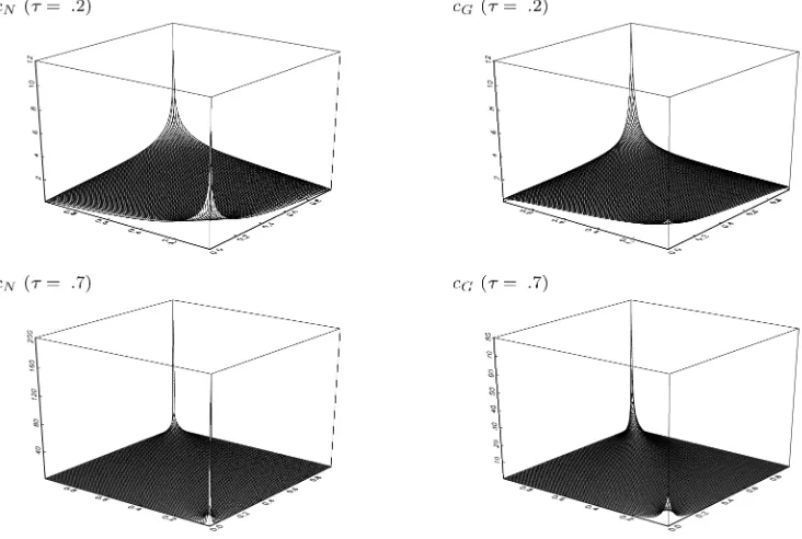
τ =.2, .7 in Figure 1, and summarize the main features of this figure as follows.
First,CNandCGboth have a higher density at the 45-degree
line. This reflects the concordance implied by positiveτ’s. Sec-ond, cN(u,u;ρ) and cG(u,u;ϑ ) both increase with
increas-ing magnitude of |u−.5|. This means that the clustering ten-dency of the lower-u(upper-u) tail events increases asu→0+ (u→1−). Third, this clustering tendency increases with the strength of concordance. Fourth, cN(u,u;ρ) is symmetric to u=.5, butcG(u,u;ϑ )is asymmetric tou=.5 and has a
heav-ier upper tail. Therefore, these two copulas imply quite dif-ferent tail properties. In accordance with the shape ofcN and cG at the 45-degree line, Hu (2006) referred to CN and CG
as copulas with the U- and J-shaped dependence structures. In addition, because csG(u1,u2;ϑs)=cG(1−u1,1−u2;ϑs), ∀(u1,u2)∈ [0,1],csG is mirror-symmetric tocG about the line u1=1−u2when ϑ=ϑs. By this mirror symmetry, it should
be understood that CGs is a copula with the L-shaped depen-dence structure (heavier lower tail). Similar toCN, thetcopula
also has the U-shaped dependence structure. This terminology is useful to reflect the dissimilarities between the tail properties implied by these copulas.
Figure 1. The normal and Gumbel copula density functions.
To characterize such tail properties more formally, we also define the lower-utail-dependence measure by the conditional probability
λL(u):=P(A1L(u)|A2L(u))=
Co(u,u)
u , u∈(0, .5],
and the upper-u tail-dependence measure by the conditional probability
λU(u):=P(A1U(u)|A2U(u))
=C
s
o(1−u,1−u)
1−u , u∈ [.5,1),
whereCso is the survival copula ofCo, andCo is temporarily
assumed to be static under assumption A. Note thatCs(1−u, 1−u)=1−2u+C(u,u)=1
u
1
u c(u1,u2)du2du1. It is easy
to see thatλL(u)andλU(u)are invariant to the replacements
ofA2L(u)|A1L(u)andA2U(u)|A1U(u)and are bounded in[0,1]
by the definition of probability. In fact, the Fréchet–Hoeffding inequality implies that the ratios C(u,u)/u and Cs(1 −u, 1−u)/(1−u)are always bounded in[0,1]for any copulaC.
Given these definitions, the lower-u tail events are inde-pendent if and only ifλL(u)=u, that is,P(A1L(u)|A2L(u))= P(A1L(u)). On the other hand, the upper-u tail events are
in-dependent if and only if λU(u)=1−u. In contrast, the
in-equality λL(u)=u [λU(u)=1−u] implies the dependence
of lower-u (upper-u) tail events. Clearly,Co=CI implies no
tail dependence for anyu. Figure 2, shows the implied differ-encesλL(u)−u andλU(u)−(1−u)of Co=CN,Co=CG, Co=CGs, and Co=Ct with τ =.2, .7. This figure indicates
that these differences are all positive ifu=0 andu=1. In other words, they imply both lower and upper tail dependence except for the extreme cases whereu=0,1. For these two extreme
(a) (b)
Figure 2. The differences (a)λL(u)−uand (b)λU(u)−(1−u)implied byCN,Ct,CG, andCsG.
cases, we haveλ∗L:=limu→0+λL(u)andλ∗U:=limu→1−λU(u),
which measure the lower extreme-value dependence and the upper extreme-value dependence (see, e.g., Joe 1997). It is known thatCo=CN implies that λ∗L=λ∗U =0. In compari-et al. 2003; Schmidt 2004). Some studies refer to a copula with λ∗L=0 (λ∗U=0) as a “lower tail–independent” (“upper tail– independent”) copula, but this terminology ignores the differ-ence between the tail events and the extreme events. To avoid the resulting ambiguity, in this study we distinguish tail depen-dence from extreme-value dependepen-dence and measure the former byλL(u)andλU(u)and the latter byλ∗Landλ∗U.
This discussion demonstrates thatCN,CG,CsG, andCt are
all capable of interpreting concordance but may have quite different tail-dependence, extreme-value dependence, or both structures. The literature reports many other parametric copu-las; for example, the Frank copula has a U-shaped dependence but no extreme-value dependence, and the Clayton copula has an L-shaped dependence and lower extreme-value dependence, and the Clayton-survival copula has a J-shaped dependence and upper extreme-value dependence. We may even accommodate various cross-dependence structures by using a mixed copula that combines different copulas with different weights (see, e.g., Hu 2006). TheMtest can be applied to any of these parametric copulas. Nevertheless, considering all possible copulas in em-pirical studies seems impracticable. It would be more reason-able to consider certain sensible representative ones and then check whether these copulas need to be respecified. TheMtests with properly selectedφ’s are useful for this task.
Following Jondeau and Rockinger (2006) and Patton (2006a), we can easily extend our discussions to dynamic copulas by specifying the copula parameters as certain dynamic functions of xt. Specifically, we can define the dynamic normal copula CN(u1,u2|xt;θ )using the DCC coefficientρt=ρt(xt;θ ), such
as that of Tse and Tsui (2002),
ρt=(1−κ1−κ2)κo+κ1ρt−1
staticCGandCsG, we can also define the dynamic Gumbel
cop-ulaCG(u1,u2|xt;θ )and the dynamic Gumbel-survival copula CsG(u1,u2|xt;θ ). Similarly, we can define the dynamictcopula Ct(u1,u2|xt;θ ) using the same ρt to replace the CCC
coeffi-cient ρ of Ct(u1,u2;ρ, ν). By fixing the same ρt, these
dy-namic copulas have the same dydy-namic Kendall’s tauτ (xt;θ )in the population but still have different tail-dependence struc-tures characterized by the dynamic lower-u tail-dependence measuresλL(u|xt;θ )=u1C(u,u|xt;θ )and the dynamic upper-u
tail-dependence measuresλU(u|xt;θ )=1−1uCs(1−u,1−u|xt;
θ )for variousC’s. These dynamic copulas degenerate to the sta-tic counterparts asρt=ρfor all of thet’s. The tests introduced
next are applicable to both the static and dynamic copulas.
3.2 Concordance Test and Tail-Dependence Tests
By definition, it is easy to see that the condition E[φot| It−1] =0 is satisfied for all of the followingφ’s:
ty–associated parametersηcoandηio, using their sample
coun-terparts. Given these estimators, the transformationϕˆt in (14),
and thus theMτ test statistic, are immediately computable.
For theML(u) test with some u∈(0, .5], we have∇θ⊤φt=
pothesis. Following the same argument, it is easy to see that
E[pitfitεitz⊤it] = −
tations are free of the Dirac delta function and thus can be esti-mated directly using their sample counterparts in practical ap-plications. Given the estimators ofE[∇θ⊤φt]and these expec-tations, theML(u)test becomes immediately applicable.
For theMU(u) test with someu∈(.5,1], we have∇θ⊤φt=
hypothesis. Given the estimators ofE[∇θ⊤φt]and these
expec-tations, theMU(u)test is applicable.
TheMτ,ML(u), andMU(u)tests are designed to check the
cri-teria of concordance, lower-utail dependence, and upper-utail dependence individually. These individual tests are expected to be powerful against the copula misspecifications in the direc-tions of concordance, lower-utail dependence, and upper-utail dependence; thus they are useful for identifying the possible causes of copula misspecification and refining the misspecified copula. In financial applications, theMτtest also may be used to
evaluate the adequacy of the copula in characterizing the mar-ket comovements in normal times. Some studies have checked the VaR validation using a graphical comparison between the observed tail frequencies and the theoretical tail probabilities, implied by the copula used to evaluate VaR, at different confi-dence levelsu∈(0,1)(see, e.g., Cherubini and Luciano 2001). Clearly, theML(u)andMU(u) tests formalize such a
graphi-cal comparison method, and the indexumay be interpreted as the associated confidence level. As such, these tail-dependence tests should be particularly useful for evaluating the VaR vali-dation and the related risk-management applications.
This demonstrates some potential importance and applicabil-ity of these individual tests. Nonetheless, it is quite possible that a misspecified copula may satisfy the criterion of concordance but fall short of certain tail-dependence criteria, as implied by the discussion in Section 3.1 and as we show in the simulation. Similarly, it is also possible that a misspecified copula may sat-isfy the tail-dependence criterion for certainu’s but fail to sat-isfy this criterion for other u’s. Therefore, in addition to the individual tests, it is also important to evaluate various criteria simultaneously. In our approach we can easily establish such a test by basing theMtest on certain multidimensional testing in-dicators. In particular, we may base theMtest on the following 2p-dimensionalφ:
φLU:=φL(v1), . . . , φL(vp), φU(1−vp), . . . , φU(1−v1) ⊤
, (26)
for some vi ∈(0, .5), vi<vi+1, and i=1,2, . . . ,p. We re-fer to this test as the MLU test. The MLU test statistic can be
easily computed by redefining the transformation ϕˆt in (14)
as a 2p ×1 vector composed of the ϕˆt’s implied by the ML(v1), . . . ,ML(vp),MU(1−vp), . . . ,andMU(1−v1)tests. This test statistic has the asymptotic null distributionχ2(2p). Unlike the aforementionedMtests, theMLUtest can check the copula
mis-specifications for various tail-dependence structures simultane-ously.
In addition, we can also easily extend theMτ,ML(u),MU(u),
andMLUtests to the multivariate copula tests by replacing the
bivariate Kendall’s tau and tail-dependence measures with their multivariate generalizations. Specifically, as noted by Nelsen (2002), the bivariate Kendall’s tau in (19) has a multivariate generalization,
base the multivariate concordance test on the testing indicator
φτ(ut|xt;θ )=
variate copula with then-dimensional copula, we can also de-fine the multivariate tail-dependence measures λL(u|xt;θ )= 1
uC(u,u, . . . ,u|xt;θ )andλU(u|xt;θ )= 1 1−uC
s(1−u,1−u, . . . ,
1−u|xt;θ )and base the multivariate tail-dependence tests on the extendedφL(u)andφU(u),
These multivariate copula tests degenerate to the bivariate cop-ula tests whenn=2.
For the multivariate tail-dependence tests, the expectations
E[pitfitw⊤it],E[pitfitεitz⊤it], andE[pitFit]are of the same forms
as those in the bivariate case, but the transformationsduitandeuit must be generalized asditu=u
also Cherubini, Luciano, and Vecchiato 2004, p. 142, for more discussions regarding the multivariate survival copula.)
As pointed out by a referee, it also may be noteworthy that, using the standardized residuals vectorεt to replace the PITs
vectorut in the testing indicatorφt and applying the
general-ized first-order asymptotics to rederive the asymptotic distribu-tion of the resulting “√TDˆT,” we also might establish a class of
moment-based tests for the entire multivariate conditional den-sity model composed of the marginal models and the copula model. Similar to the concordance and tail-dependence tests, we may also base this class of tests on the correlation coef-ficients ofεt or the conditional quantile exceedances ofεt to
check the entire multivariate conditional density model in vari-ous directions. To focus on testing the copula model, we do not further pursue the details of this testing approach in the rest of this article.
4. MONTE CARLO SIMULATION
In this simulation we assess the finite-sample performance of the proposed method. The CMD model being tested is of the form
Table 1. Empirical sizes and powers of theMτtest
Ho:Co=CI Ho:Co=CN CI(uncorrected) CN(uncorrected) Co T=500 1,000 2,500 T=500 1,000 2,500 T=500 1,000 2,500 T=500 1,000 2,500
CI 8.1 7.4 6.6 7.0 6.8 7.9 0 0 0 0 0 0
CN(τ1) 43.8 68.7 95.8 6.8 8.5 7.6 .2 2.9 31.4 0 0 0
CN(τ2) 100.0 100.0 100.0 7.6 8.4 7.5 100.0 100.0 100.0 0 0 0
CG(τ1) 43.4 70.8 96.6 7.5 6.7 8.3 .1 2.6 27.5 0 0 0
CG(τ2) 100.0 100.0 100.0 7.3 9.3 7.2 100.0 100.0 100.0 0 0 0
Ct(τ1) 38.2 61.2 94.6 6.4 8.1 5.8 .2 2.8 28.6 0 0 0
Ct(τ2) 100.0 100.0 100.0 7.8 9.2 9.4 100.0 100.0 100.0 0 0 0
NOTE: The bold entries represent the empirical sizes in percentages; the others are the empirical powers in percentages. The “uncorrected” blocks correspond to the tests without the correction for estimation uncertainty.
αh2(yi,t−1 −mi,t−1)2, and the iid N(0,1) standardized er-ror εit for both i=1,2. The copula model being tested
in-cludesC=CI and the staticCN, and the true copula includes Co=CI, CN, CG, and Ct with the static parameter ρ=.1
and .5 (or, equivalently, the static Kendall’s tau τ1:=.0638 andτ2:=.3317), whereCt has the degrees of freedomν=4.
The marginal models are set to be correctly specified in the sense of assumption A with (αmo, αm1, αho, αh1, αh2)= (.01, .05, .05, .85, .1). This experimental design essentially fol-lows that of Chen et al. (2004).
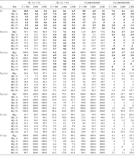
Given T =500, 1,000, 2,500, the 5% nominal level, and 1,000 replications, we present the empirical sizes and powers of theMτtest in Table 1 and give the simulation results of theMLU
test with(v1,v2,v3,1−v3,1−v2,1−v1)=(.1, .3, .5, .5, .7, .9) and the associatedML(u)andMU(u)tests in Table 2. To
demon-strate the importance of correcting the effect of estimation un-certainty, we also report the empirical sizes and powers of the uncorrected tests in these two tables. Specifically, these uncor-rected tests standardize the statistic√TDˆT=T−1/2Tt=1φˆt
us-ing the sample counterpart ofE[φotφot]⊤ , rather than the
esti-mator of the estimation uncertainty–corrected asymptotic vari-anceo.
From these two tables, it can be seen that these uncorrected tests are substantially undersized in most cases. Importantly, this distortion may not be remedied, but instead may be dam-aged, by the increase inT. In contrast, the empirical sizes of the M test are quite close to the 5% nominal level for both the continuously differentiable testing indicatorφτ and the
dis-crete testing indicatorsφL(u) and φU(u) and for both the
one-dimensional testing indicatorsφτ,φL(u), andφU(u)and the
mul-tidimensional testing indicatorφLU. A mild exception appears
in the case where theMLU,ML(.1), andMU(.9)tests have the
empirical sizes 10.9%, 10.1%, and 11.6% whenCo=CI and T=500. Nonetheless, this distortion disappears asT=1,000. This size performance not only demonstrates the importance of correcting the estimation uncertainty effect, but also supports the validity of the generalized first-order asymptotics used in Section 2.
These two tables also show that the empirical powers of the uncorrected tests are generally smaller than those of the cor-rected tests. In addition, the M tests have quite good perfor-mance against the copula misspecifications that they are de-signed to detect. The empirical powers of theMτ test against
the misspecifiedCI increase rapidly with the Kendall’s tau of Co and the sample size, regardless of whetherCo=CN, CG,
orCt. This means that this test can successfully capture the
con-cordance structures ignored byCI. Interestingly, the empirical
“powers” of theMτ test against the misspecifiedCNare close
to (or slightly greater than) the 5% level in both cases where Co=CGandCo=Ct. This is quite a reasonable result because
it reflects the fact thatCNis also capable of interpreting the
con-cordance structure implied byCGandCt. Nevertheless, it also
reminds us that we should not rely completely on the concor-dance test to conclude the adequacy of the copula, as discussed in Section 3.2.
Indeed, what CN cannot interpret are the tail-dependence
structures ofCGandCt. As expected, theMLUtest is quite
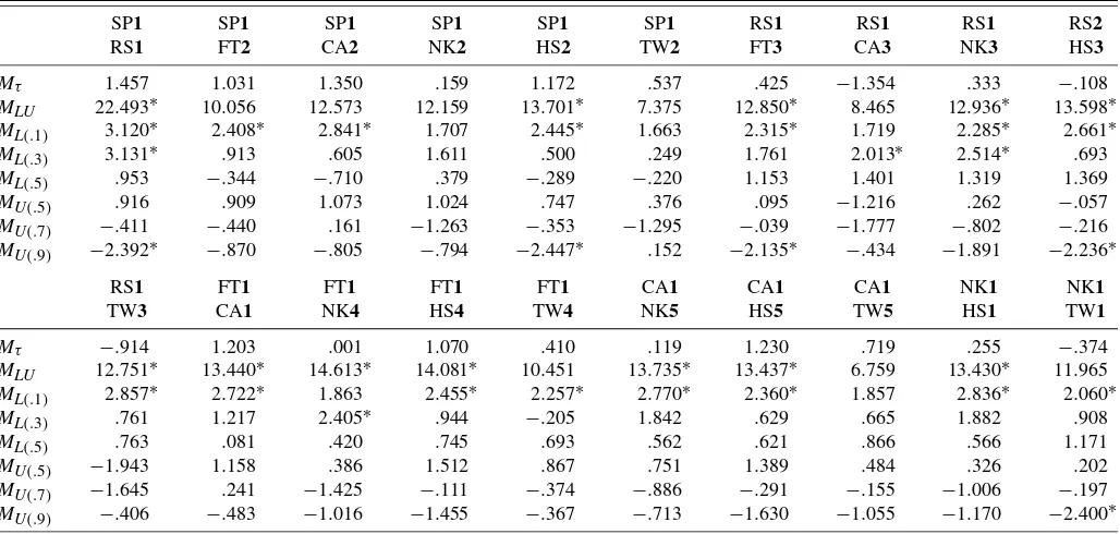
pow-erful in these directions. Table 2 shows that, givenT=2,500, theMLUtest is of empirical power 99.8% against the
misspec-ifiedCN when Co=CG andτ =τ2 and has empirical power 99.1% against the misspecifiedCN whenCo=Ct andτ =τ1. This shows that the MLU test can successfully discriminate
between copulas with different tail dependence structures for properT’s andτ’s.
Table 2 also shows that, given τ =τ2 and T=2,500, the ML(.1),ML(.3),ML(.5),MU(.5),MU(.7), andMU(.9)tests are
of empirical powers 70.6%, 47.7%, 5.7%, 6.2%, 65.2%, and 99.5% against the misspecifiedCN when Co=CG. Quite
re-markably, this J-shaped power performance is consistent with the dissimilarity between the J-shaped dependence ofCo=CG
and the U-shaped dependence of CN, as discussed in
Sec-tion 3.1; see also Figure 2 for an explanaSec-tion why theMU(.9)
test has a higher power than theML(.1)test. Givenτ =τ1and T=2,500, these tests are of empirical powers 84.8%, 14.9%, 5.8%, 5.8%, 16.1%, and 84.6% against the misspecified CN
when Co=Ct. This U-shaped performance is also consistent
with the symmetric lower and upper extreme-value dependence ofCo=Ctthat cannot be interpreted byCN. Such a power
per-formance is quite encouraging, demonstrating the usefulness of the proposed individual tests in shedding light on the possible directions of copula misspecification. This property is impor-tant because Co is unknown in practical applications, and we
must identify the possible causes of mis-specification before re-specifying the misspecified copula model.
Theoretically, we cannot completely and fairly compare our tests with the density estimate–based tests of Chen et al. (2004) on the same basis, because those tests are based on differently designed contexts. Unlike our tests, their tests are designed for the semiparametric CMD context that replaces the parametric standardized error distribution Fεi(·|xt;βi) with the empirical
Table 2. Empirical sizes and powers of theMLU,ML(u), andMU(u)tests
Ho:Co=CI Ho:Co=CN CI(uncorrected) CN(uncorrected) Co Test T=500 1,000 2,500 T=500 1,000 2,500 T=500 1,000 2,500 T=500 1,000 2,500
CI MLU 10.9 6.6 5.6 8.2 8.1 6.5 8.9 4.9 3.1 7.6 4.1 2.1
ML(.1) 10.1 6.2 6.0 7.4 6.0 5.5 9.5 5.8 3.0 6.6 4.8 3.0
ML(.3) 5.5 4.7 5.4 5.8 4.3 5.9 1.9 2.2 2.3 .7 .8 1.2
ML(.5) 6.5 5.7 5.7 5.6 5.2 4.9 1.7 .7 1.6 .7 .4 .4
MU(.5) 5.2 5.9 4.6 6.5 5.2 5.6 1.7 1.3 .9 .4 .3 .3
MU(.7) 5.5 6.6 5.8 4.2 4.2 5.2 2.1 2.5 2.0 1.0 .4 1.3
MU(.9) 11.6 6.3 5.0 7.6 6.6 4.8 11.1 5.7 2.5 7.4 5.7 3.4
CN(τ1) MLU 19.1 38.1 86.0 7.3 7.1 5.6 11.9 26.9 77.6 5.2 3.7 1.5
ML(.1) 8.4 12.1 34.3 5.4 4.5 5.1 5.0 7.1 27.8 4.3 3.2 2.9
ML(.3) 20.5 34.2 70.6 5.0 5.0 5.0 9.1 17.9 53.6 .4 .7 .6
ML(.5) 21.2 36.7 69.1 5.2 6.1 5.7 6.5 16.5 44.2 .8 .2 .3
MU(.5) 17.6 32.1 68.1 5.1 6.2 5.8 5.0 12.8 43.7 .5 .7 .3
MU(.7) 18.8 33.7 69.9 5.5 6.0 5.1 7.3 19.3 53.9 .9 .7 .2
MU(.9) 9.5 13.1 33.6 5.7 6.6 5.2 6.5 8.9 26.1 4.8 4.1 2.5
CN(τ2) MLU 100.0 100.0 100.0 6.2 6.3 4.9 100.0 100.0 100.0 2.5 1.7 1.2
ML(.1) 96.8 99.9 100.0 6.9 5.3 3.8 92.0 99.9 100.0 2.4 1.8 1.0
ML(.3) 100.0 100.0 100.0 5.8 5.6 4.9 100.0 100.0 100.0 .6 .5 .6
ML(.5) 100.0 100.0 100.0 5.3 5.6 5.8 100.0 100.0 100.0 .4 .2 .3
MU(.5) 100.0 100.0 100.0 5.0 6.0 5.4 99.9 100.0 100.0 .3 .3 0
MU(.7) 100.0 100.0 100.0 4.0 5.9 6.5 100.0 100.0 100.0 0 .3 .7
MU(.9) 96.1 100.0 100.0 5.2 5.5 5.0 92.8 99.9 100.0 2.1 1.9 .8
CG(τ1) MLU 24.6 52.6 97.1 8.4 12.8 25.9 14.0 35.2 92.1 5.6 6.1 11.5
ML(.1) 7.1 7.1 18.8 9.8 8.6 10.8 5.2 3.7 14.2 9.1 7.1 8.0
ML(.3) 12.7 23.8 52.0 6.5 9.5 10.6 4.4 10.8 36.1 1.1 2.6 2.1
ML(.5) 18.6 33.4 65.2 4.7 5.4 5.5 7.6 14.9 40.7 .2 .5 .2
MU(.5) 18.3 31.8 65.1 5.3 6.3 6.0 7.0 13.3 38.9 .6 .3 .3
MU(.7) 29.9 52.0 88.3 5.9 7.8 9.2 11.9 31.7 75.9 .8 .8 1.3
MU(.9) 24.5 48.5 92.8 9.5 16.5 42.9 13.9 38.3 89.5 3.4 5.9 25.7
CG(τ2) MLU 100.0 100.0 100.0 45.4 79.3 99.8 100.0 100.0 100.0 15.9 35.7 88.7 ML(.1) 77.5 97.5 100.0 19.9 34.5 70.6 66.5 95.5 100.0 13.7 24.0 55.1 ML(.3) 100.0 100.0 100.0 15.9 23.2 47.7 99.5 100.0 100.0 2.3 5.0 16.0
ML(.5) 100.0 100.0 100.0 4.6 5.9 5.7 99.8 100.0 100.0 .2 .1 .1
MU(.5) 100.0 100.0 100.0 5.7 5.9 6.2 100.0 100.0 100.0 .1 .4 .8
MU(.7) 100.0 100.0 100.0 18.4 31.1 65.2 100.0 100.0 100.0 1.6 4.9 20.7
MU(.9) 100.0 100.0 100.0 50.4 85.0 99.5 100.0 100.0 100.0 17.8 55.9 97.5
Ct(τ1) MLU 43.7 88.7 100.0 22.8 61.5 99.1 24.1 74.9 99.9 4.2 13.4 69.5
ML(.1) 40.3 72.7 99.2 17.9 38.0 84.8 27.2 64.3 98.6 5.4 21.7 71.5
ML(.3) 31.4 54.3 93.0 8.6 8.3 14.9 13.4 33.5 84.2 .8 1.2 2.6
ML(.5) 23.1 35.0 70.7 7.1 6.1 5.8 8.5 15.3 44.3 .6 .3 .5
MU(.5) 18.2 31.4 67.0 5.5 6.2 5.8 6.4 12.3 41.9 .5 .3 .4
MU(.7) 31.2 53.5 92.6 7.8 10.0 16.1 14.0 32.3 82.1 1.3 1.3 2.3
MU(.9) 41.7 71.6 98.9 18.7 41.2 84.6 28.9 62.7 98.2 8.4 23.3 71.6
Ct(τ2) MLU 100.0 100.0 100.0 19.2 37.3 89.2 100.0 100.0 100.0 4.1 4.7 24.7 ML(.1) 99.4 100.0 100.0 14.1 24.5 63.6 99.1 100.0 100.0 2.6 7.7 35.2
ML(.3) 100.0 100.0 100.0 7.2 8.9 14.2 99.9 100.0 100.0 .8 .5 1.7
ML(.5) 100.0 100.0 100.0 6.4 5.0 7.6 99.9 100.0 100.0 .3 .5 .6
MU(.5) 100.0 100.0 100.0 5.0 5.9 5.5 99.6 100.0 100.0 .1 0 .2
MU(.7) 100.0 100.0 100.0 7.3 8.5 15.3 100.0 100.0 100.0 .5 .9 2.3
MU(.9) 99.7 100.0 100.0 14.2 27.0 61.8 99.3 100.0 100.0 2.7 7.1 35.0
NOTE: The bold entries represent the empirical sizes in percentages; the others are the empirical powers in percentages. The “uncorrected” blocks correspond to the tests without the correction for estimation uncertainty.
distribution function of the standardized residualεˆit’s. Because
the parametric and semiparametric modeling approaches both exist in the copula studies, these two classes of tests may have different potential applications and should not be exclusive to each other. Nonetheless, we may still discuss the performance
of the tests, which is to some extent based on the same simula-tion design.
Chen et al. (2004) introduced two density estimate–based tests: test 1, a multivariate density estimate–based consistent test, and test 2, a univariate density estimate–based
tent test. By basing on some particular choices of kernel and bandwidth, their simulation shows that givenT=500, 2,500, and 5,000, test 1 (test 2) has empirical sizes 0%, .4%, and 5.2% (.4%, 2.0%, and 3.2%) under the null hypothesisCo=CNwhen
ρ=.1 and the empirical sizes 0%, 2.4%, and 4.0% (1.6%, 2.4%, and 2.4%) asρ=.5; see Chen et al.’s tables 5 and 6. This indicates that although the density estimate–based tests are asymptotically free of the standardized error distribution speci-fications, they could be obviously undersized in small and mod-erate samples. In comparison, although the moment-based tests have much better size performance, they require correctly spec-ified standardized error distributions. Such trade-offs between the parametric and semiparametric statistical methods are com-mon. Based on these aspects, we interpret the moment-based tests as complements, rather than substitutes, to the density estimate–based tests.
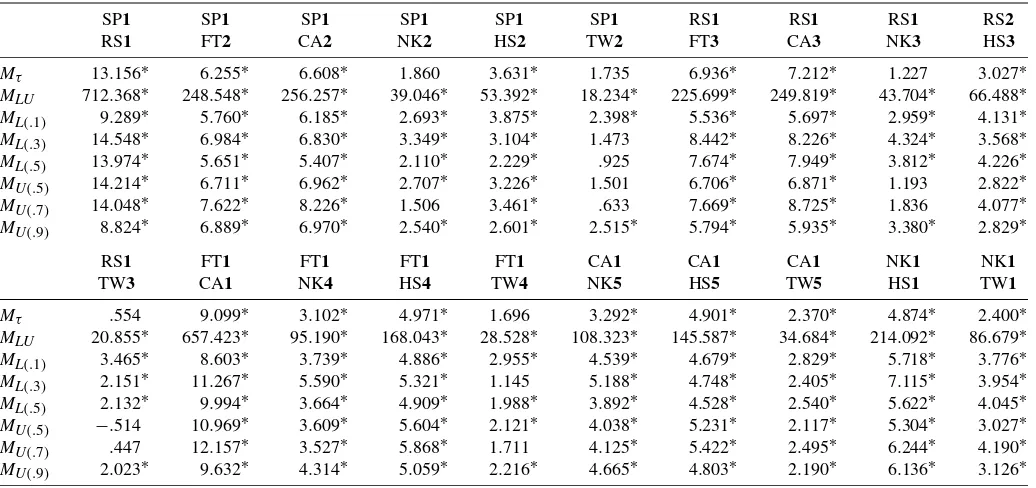
5. AN EMPIRICAL APPLICATION
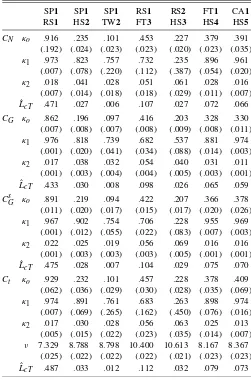
In this section we apply the concordance and tail-dependence tests to an empirical study of stock market relationships. Our discussions focus mainly on the bivariateCN,CG,CsG, andCt,
and finally extend to the trivariate CN and Ct. Similar to
Hu (2006), we view CN, CG, and CsG as the representative
ones with U-shaped, J-shaped, and L-shaped dependence. Re-call that thetcopula also has U-shaped dependence. If the true copula has L-shaped (J-shaped) dependence, then the cross-dependence of downside markets is stronger (weaker) than that of the upside markets. In contrast, if the true copula has U-shaped dependence, then there will be no such asymme-try. This asymmetry (symmetry) is conceptually very close to the correlation asymmetry (symmetry) studied by Longin and Solnik (2001) and Ang and Chen (2002), which is known to have important implications for portfolio diversification and risk management.
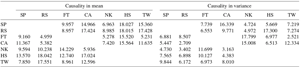
The data used in our analysis include seven major stock price indices: the Standard & Poor 500 (SP) and Russell 2000 (RS) of the United States, the Financial Times Stock Exchange 100 (FT) of the United Kingdom, the Compagnie des Agents de Change 40 (CA) of France, the Nikkei 225 (NK) of Japan, the Hang Seng (HS) of Hong Kong, and the Taiwan weighted (TW) for January 1, 1995–December 31, 2003. These data were obtained from Yahoo!Finance. LetPit be the closing price of
stock indexiat datetand in the local currency. This empirical study is based on the daily returns
yit=100×(lnPit−lnPi,t−1),
where t denotes the tth common calendar trading date of these markets in the sample. The sample size is T =1,915. We consider 21 pairs of returns yt =(y1t,y2t), including the
US returns SP–RS; the US–European returns SP–FT, SP–CA, RS–FT, and RS–CA; the European returns FT–CA; the Asian returns NK–HS, NK–TW, and HS–TW; the US–Asian returns SP–NK, SP–HS, SP–TW, RS–NK, RS–HS, and RS–TW; and the European–Asian returns FT–NK, FT–HS, FT–TW, CA–NK, CA–HS, and CA–TW.
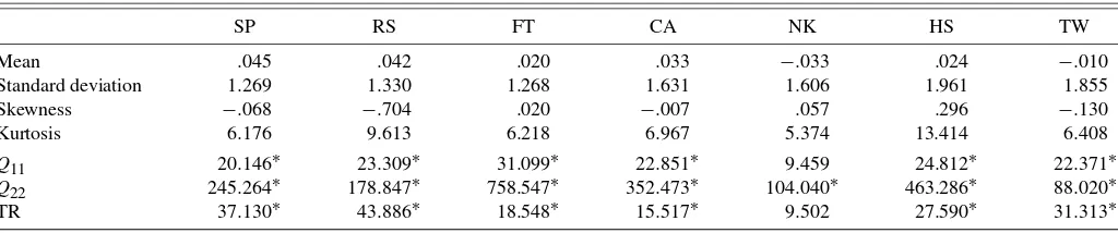
Table 3 shows the first four sample moments of returns. Not surprisingly, these returns are all leptokurtically distributed. This evidence precludes the marginal normality and hence the bivariate normality for all of the return combinations. To see whether the return series are iid, we further check the null of serial independence using the test of Ljung and Box (1978), the test of McLeod and Li (1983), and the time-reversibility (TR) test of Chen (2003). These tests are powerful against serial cor-relation, volatility clustering, and time irreversibility (asymme-try in dynamic dependence, such as the leverage effect). These power directions will provide us with useful information for es-tablishing suitable marginal models when the null of serial in-dependence is rejected. We show the test statistics in the same table and describe the tests in the footnotes to this table.
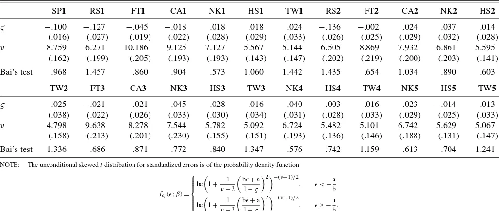
Given the 5% significance level, these tests indicate that most return series are likely to be serially correlated, volatility clus-tered, and time-irreversible. NK is the only case that has volatil-ity clustering but serial uncorrelatedness and time reversibilvolatil-ity. Nevertheless, all of these returns are dynamically dependent and need to be explained using some suitable GARCH-type models. We consider the AR–GARCH and AR–Exponential GARCH (EGARCH) models with different orders and check their adequacy using the standardized residual–based counter-parts of the Ljung–Box, McLeod–Li, and TR tests, referred to as the diagnostic tests, corrected for estimation uncertainty. Ta-ble 4, shows the Gaussian QMLEs and the diagnostic test sta-tistics of the selected GARCH-type models: SP1, RS1, FT1, CA1, NK1, HS1, and TW1. We observe that NK1 is the only case that has the GARCH specification, and the other cases all have the EGARCH specification. The diagnostic tests accept
Table 3. Descriptive statistics and serial independence test statistics
SP RS FT CA NK HS TW
Mean .045 .042 .020 .033 −.033 .024 −.010
Standard deviation 1.269 1.330 1.268 1.631 1.606 1.961 1.855
Skewness −.068 −.704 .020 −.007 .057 .296 −.130
Kurtosis 6.176 9.613 6.218 6.967 5.374 13.414 6.408
Q11 20.146∗ 23.309∗ 31.099∗ 22.851∗ 9.459 24.812∗ 22.371∗
Q22 245.264∗ 178.847∗ 758.547∗ 352.473∗ 104.040∗ 463.286∗ 88.020∗
TR 37.130∗ 43.886∗ 18.548∗ 15.517∗ 9.502 27.590∗ 31.313∗
NOTE: Letˆr1(k)be the lag-ksample autocorrelation of the return series{yt}, and denoteTk:=T−k. The Ljung–Box test statistic isQ11:=T(T+2)mk=1rˆ12(k)/Tk, and the
McLeod–Li test statisticQ22replaces{yt}inQ11with{y2t}. These two test statistics are evaluated atm=10. Under the null of serial independence, the TR test statistic TR:=
m
k=1Tkˆ′k(ˆ−2Ŵ)ˆ −1ˆk d
→χ2(m), whereˆk:=Tk−1
T
t=k+1(yt,yt−k),ˆ:=T−2Tt=1Ts=1(yt,ys)2,Ŵˆ:=T−1Tt=1[T−1Ts=1(yt,ys)]2, and(yt,yt−k):= ˜β(yt−
yt−k)/[1+ ˜β2(yt−yt−k)2], has the asymptotic null distributionχ2(m). This statistic is evaluated atβ˜=.5 andm=5 (see Chen 2003 for the finite-sample performance).∗represents significance at the 5% level. The 95% critical values ofχ2(5)andχ2(10)are 11.0705 and 18.3070.
388
Jour
nal
of
Business
&
Economic
Statistics
,
O
ctober
2007
Table 4. QMLEs of the marginal models
SP1 RS1 FT1 CA1 NK1 HS1 TW1 RS2 FT2 CA2 NK2 HS2 TW2 FT3 CA3 NK3 HS3 TW3 NK4 HS4 TW4 NK5 HS5 TW5
αmo .063 .066
(.022) (.022)
yi,t−1 .115 .040 .129 −.148 −.120 −.071 .016 −.115 −.099 −.063 .010 −.023 −.032
(.024) (.026) (.025) (.026) (.032) (.025) (.026) (.026) (.026) (.027) (.024) (.027) (.027)
yi,t−2 .069 −.032 .047 −.059 .060 .068 .070
(.026) (.022) (.027) (.023) (.025) (.025) (.025)
yj,t−1 −.035 .304 .348 .410 .475 .236 .251 .297 .363 .393 .227 .263 .269 .184 .207 .176 .160 (.022) (.024) (.045) (.030) (.033) (.037) (.023) (.030) (.032) (.031) (.034) (.033) (.031) (.035) (.025) (.025) (.027)
yj,t−2 .061 .028 −.050 −.050 .035 .056 .069
(.031) (.037) (.020) (.027) (.030) (.036) (.027)
yj,t−3 −.073 .098 .052 .094 .046
(.034) (.030) (.033) (.029) (.021)
yj,t−5 .034
(.035)
yj,t−6 −.051
(.021)
yj,t−8 −.046
(.022) αho −.064 −.113 −.079 −.075 .145 −.091 −.033 −.109 −.083 −.074 .126 −.078 −.021 −.085 −.077 .131 −.086 −.026 .138 −.086 −.037 .136 −.089 −.035
(.018) (.031) (.014) (.018) (.052) (.026) (.020) (.030) (.014) (.014) (.049) (.022) (.010) (.014) (.017) (.050) (.028) (.027) (.053) (.025) (.020) (.054) (.025) (.018) lnhi,t−i .958 .977 .983 .979 .973 .957 .979 .981 .979 .986 .990 .982 .977 .980 .926 .972 .958 .975 .965
(.007) (.010) (.004) (.006) (.009) (.012) (.009) (.004) (.006) (.005) (.005) (.004) (.007) (.007) (.019) (.009) (.012) (.008) (.011)
hi,t−i .873 .878 .876 .878 .880
(.035) (.038) (.037) (.036) (.037)
e2i,t−i .072 .068 .069 .067 .066
(.020) (.020) (.019) (.019) (.019)
εi,t−1 −.167 −.096 −.112 −.089 −.097 −.084 −.094 −.116 −.081 −.088 −.125 −.105 −.084 −.092 −.102 −.064 −.081 −.082 −.075 (.024) (.022) (.019) (.022) (.062) (.020) (.020) (.019) (.024) (.049) (.047) (.019) (.021) (.056) (.024) (.053) (.020) (.054) (.018)
|εi,t−1| .104 .157 .107 .120 .124 .109 .150 .110 .118 .135 .075 .113 .124 .188 .128 .179 .112 .158 .099
(.025) (.042) (.018) (.027) (.100) (.029) (.039) (.019) (.021) (.045) (.064) (.018) (.025) (.051) (.036) (.049) (.031) (.050) (.029)
εi,t−2 .013 .039 .020 .029 −.020 .002
(.057) (.077) (.045) (.093) (.084) (.086)
|εi,t−2| .037 −.015 .164 −.052 −.026 −.005
(.087) (.072) (.076) (.085) (.081) (.077)
εi,t−3 .061
(.096)
|εi,t−3| −.197
(.069)
y2j,t
−1 −.045 .022 −.045
(.011) (.007) (.011)
y2j,t
−2 .098 −.021 .006 .098 (.030) (.007) (.003) (.030)
Q∗11 11.644 6.269 14.143 12.451 3.679 16.721 14.780 6.065 17.350 14.041 12.676 18.266 13.849 13.834 13.505 12.029 17.707 13.351 10.812 17.610 9.630 13.402 16.696 8.667 Q∗22 9.031 11.233 8.304 8.710 14.640 9.387 10.675 10.468 7.618 7.294 8.397 13.478 12.089 6.481 5.959 12.867 12.638 12.607 10.632 11.518 12.635 11.093 10.563 15.067 TR∗ 2.055 10.125 4.866 7.201 9.829 7.865 9.555 10.385 3.122 5.539 3.230 3.194 9.266 3.980 7.266 5.366 5.469 8.237 8.232 4.969 9.991 5.833 5.555 9.149 Kiefer–
Salmon 115.859 1,424.243 103.775 289.372 352.394 593.794 843.573 1284.299 203.936 892.647 518.037 582.132 898.081 157.237 413.149 506.394 603.496 1,113.570 311.382 583.099 940.772 349.734 510.009 944.371 Skewness −.165 −.795 .063 .081 −.081 −.134 −.134 −.775 .135 .216 −.058 .015 −.232 .147 .150 −.076 −.067 −.197 .028 −.120 −.153 −.030 −.150 −.219 Kurtosis 3.960 6.893 4.081 4.859 5.069 5.718 6.224 6.678 4.513 6.275 5.515 5.730 6.240 4.333 5.209 5.488 5.774 6.712 4.933 5.700 6.404 5.060 5.534 6.394 NOTE: The entries (in parentheses) are the first-stage Gaussian QMLEs (and their standard deviations) of the GARCH-type models:mit=0,hit=heit:=exp(αho+αh1lnhi,t−1+αh2εi,t−1+αh3|εi,t−1|)for SP1, CA1, and FT1;mit=αmo+αm1yi,t−1; hit=heitfor RS1;mit=αm1yi,t−1,hit=exp(αho+αh1lnhi,t−1+αh2εi,t−1+αh3|εi,t−1| +αh4εi,t−2+αh5|εi,t−2|)for HS1;mit=αm1yi,t−2,hit=heitfor TW1;mit=0,hit=hgit:=αho+αh1hi,t−1+αh2e2i,t−1, whereeit:=yit−mit, for NK1;mit=
αmo+αm1yi,t−1+αm2yj,t−1,hit=heit, whereyjtdenotes the HS return, for RS2;mit=αm1yi,t−1+αm2yi,t−2+αm3yj,t−1,hit=heit, whereyjtdenotes the SP return, for FT2;mit=αm1yi,t−1+αm2yj,t−1+αm3yj,t−3,hit=heit, whereyjtdenotes the SP
return, for CA2;mit=αm1yj,t−1,hit=hgit, whereyjtdenotes the SP return, for NK2; andmit=αm1yi,t−1+αm2yj,t−1+αm3yj,t−2+αm4yj,t−3,hit=exp(αho+αh1lnhi,t−1+αh2εi,t−1+αh3|εi,t−1| +αh4εi,t−2+αh5|εi,t−2| +αh6y2j,t−1+αh7y2j,t−2), whereyjtdenotes the SP return, for HS2other models are similarly defined. See the Appendix for the estimation method. The test statisticsQ∗11,Q∗22, and TR∗are the standardized residual–based diagnostic test statistics corresponding to the original returns–based test statisticsQ11,Q22, and TR shown in Table 3 with the correction for estimation uncertainty (see Chen 2003 for the TR test and Chen 2007 for theQ∗11andQ∗22tests). Under the null of conditional normality, the Kiefer–Salmon test statistic is of the formT6(μˆ3−3μˆ1)2+24T(μˆ4−6μˆ2+3)2
d
→χ2(2), whereμˆi:=T−1Ti=1εˆit, andεˆtdenotes the standardized residuals; as discussed by Bontemps and Meddahi (2005), this test is applicable to the standardized residuals of the GARCH-type models. “Skewness” and “kurtosis” represent the sample skewness and kurtosis coefficients of the standardized residuals.