Full Terms & Conditions of access and use can be found at
http://www.tandfonline.com/action/journalInformation?journalCode=ubes20
Download by: [Universitas Maritim Raja Ali Haji] Date: 12 January 2016, At: 23:23
Journal of Business & Economic Statistics
ISSN: 0735-0015 (Print) 1537-2707 (Online) Journal homepage: http://www.tandfonline.com/loi/ubes20
Gradients in Spatial Response Surfaces With
Application to Urban Land Values
Anandamayee Majumdar, Henry J Munneke, Alan E Gelfand, Sudipto
Banerjee & C. F Sirmans
To cite this article: Anandamayee Majumdar, Henry J Munneke, Alan E Gelfand, Sudipto
Banerjee & C. F Sirmans (2006) Gradients in Spatial Response Surfaces With Application to Urban Land Values, Journal of Business & Economic Statistics, 24:1, 77-90, DOI: 10.1198/073500105000000162
To link to this article: http://dx.doi.org/10.1198/073500105000000162
Published online: 01 Jan 2012.
Submit your article to this journal
Article views: 72
View related articles
Gradients in Spatial Response Surfaces With
Application to Urban Land Values
Anandamayee MAJUMDAR
Department of Mathematics and Statistics, Arizona State University, Tempe, AZ 85287
Henry J. MUNNEKE
Terry College of Business at the University of Georgia, Athens, GA 30602
Alan E. GELFAND
Institute of Statistics and Decision Sciences, Duke University, Durham, NC 27708 (alan@stat.duke.edu)
Sudipto BANERJEE
Division of Biostatistics, University of Minnesota, Minneapolis, MN 55455
C. F. SIRMANS
Center for Real Estate and Urban Economic Studies, University of Connecticut, Storrs, CT 06269
For point-referenced spatial data, we often create explanatory models that introduce regression structure with error consisting of a spatial term and a white noise term. Here we consider more flexible regres-sion structures that allow spatially varying regresregres-sion coefficients. The resulting mean becomes a spatial response surface that is a linear combination of the components of the spatially varying coefficient vec-tor. Of possible interest in this setting would be gradients associated with the coefficient surfaces as well as the mean surface. Gradients could be sought at arbitrary points and in arbitrary directions. Extending ideas developed in earlier work, we obtain a fully inferential approach within the Bayesian framework for examining such gradients. In particular, we can obtain posterior distributions for any such gradient, for the direction of maximal gradient, and for the magnitude of the maximal gradient. The motivation for our work is the desire to examine urban land value gradients. There is considerable literature in the real estate community on economic theory, modeling, and data analysis relating urban land values to distance from the city center. Here we focus on gradients to such surfaces. The flexibility of our approach allows for much richer insights into the behavior of such gradients than was available previously. We illustrate by fitting a portion of Olcott’s classic Chicago land value data.
KEY WORDS: Bayesian framework; Coregionalization; Directional derivative; Finite-directional dif-ference; Markov chain Monte Carlo; Multivariate spatial process.
1. INTRODUCTION
Consider point-referenced spatial data that we assume (per-haps after suitable transformation) to be normally distributed. So we use a Gaussian spatial process to specify the joint distri-bution for an arbitrary number of and arbitrary choice of loca-tions in some region of interest, leading to a model of the form
Y(s)=XT(s)β˜(s)+ǫ(s), (1) whereǫ(s)are iid N(0, τ2), whereX(s)isp×1 and includes an intercept and β˜(s) follows a multivariate Gaussian spatial process model. The model in (1) has been referred to as a spa-tially varying coefficient model (Gelfand, Kim, Sirmans, and Banerjee 2003). For each explanatory variable, it allows the possibility of a coefficient surface over the study region rather than restriction to a constant coefficient. Instead of specify-ing these surfaces parametrically (as in, e.g., Luo and Wahba 1998), we model them as realizations from dependent spatial processes.
The mean can be removed from each coefficient process to rewrite the model as
Y(s)=XT(s)β+XT(s)β(s)+ǫ(s), (2) where now β(s) is a mean-0 multivariate Gaussian process. Thus β can be interpreted as a global coefficient vector
withβ(s)providing local variation aroundβ. In particular, the spatially varying intercept inβ(s)can be viewed as a familiar spatial random effect which, along withǫ(s), would yield a cus-tomary residual at location s. Gelfand et al. (2003) noted that XT(s)β(s)+ǫ(s)in (2) could be viewed as a residual with the first piece interpreted as a spatial component and the second as a pure error component.
In this article our interest is in the analysis of directional gra-dients associated with the response surface,XT(s)β˜(s), or with the components of β˜(s). Recent work by Banerjee, Gelfand, and Sirmans (2003) has addressed the problem of the rate of change of a spatial surface at a given point in a given direction. In their development they formalized the notion of a directional derivative spatial process associated with a univariate spatial process. Here our contribution is to extend their ideas to di-rectional gradients associated with linear combinations of mul-tivariate processes, for example, the univariate spatial process XT(s)β˜(s). In this article such gradients are associated with expected land value surfaces. However, there are many other applications where such mean surface gradients would be of
© 2006 American Statistical Association Journal of Business & Economic Statistics January 2006, Vol. 24, No. 1 DOI 10.1198/073500105000000162
77
interest, including estimated weather surfaces, such as for tem-perature or precipitation; estimated pollution surfaces, such as for ozone or particulate matter; estimated risk surfaces reflect-ing risk for a particular adverse health outcome. Again, the mean surface provides a global or first-order description of the process guiding the data, whereas gradient analysis provides a local or second-order analysis to enhance our understanding of the nature of the mean surface. Directional finite differences are frequently studied in this regard and are, in fact, routinely avail-able in GIS software packages. Infinitesimal gradients may be more attractive in avoiding specification of and possible stabil-ity issues with the scale of the finite difference. Moreover, if a model choice criterion selects a model with mean surface as in (2), then gradient analysis should be investigated under the chosen model.
Evidently, smoothness of response surface realizations is re-quired to ensure the general existence of directional derivatives. Fortunately, smoothness of spatial process realizations can be secured through specification of the covariance function. The choice of covariance function to provide almost sure continuity of process realizations has been discussed by Kent (1989). For our purposes, we require mean square differentiability (Stein 1999), which is connected to the existence of a second deriva-tive at the origin for the covariance function. We briefly review the development of a directional derivative process in Section 4 (and give relevant distribution theory in App. A).
Again, the motivation for our work is interest in urban land value gradients. There is a considerable theory and literature on urban land economics that focuses on the structure of land values, with particular emphasis on gradients; this material is reviewed in Section 2. For instance, the monocentric city model predicts that urban land values decline with distance from the central business district (CBD). Negative exponential decay has theoretical support (Mills 1972; Muth 1969); however, the land value function has become more complex over time. In some parts of a city, land values may in fact increase with increasing distance from the CBD. Moreover, gradients to the land value surface may depend on direction. Models such as (2) allow us to accommodate both of these features. The former is achieved by allowingX(s)to include other determinants of land value, such as distances to other externalities or amenities specific to the urban area. X(s)may also reflect amenities at location s, such as quality of local schools, crime levels, or environmental quality. The latter is enabled by the spatially varying form for theβ˜(s), which allows us to formalize a gradient at a location in a given direction. As a result, we can look at gradients to the land value function at arbitrary points, in arbitrary directions.
Here we offer a fully inferential framework to examine such gradients. Because none of the components ofβ˜(s), and hence of XT(s)β˜(s), are observed, inference about associated gradi-ents is arguably most easily implemented within a Bayesian framework. Thus entire posterior distributions can be supplied for the magnitude of any particular directional gradient. Fur-thermore, because at a given location, for a given surface, we can identify the direction of maximal gradient and the magni-tude of the gradient in that direction, posteriors for these un-knowns also can be obtained. Development of the theory and modeling for such a Bayesian setting is laid out in Section 5. Computational details are described there as well as in Appen-dix A. Section 6 and AppenAppen-dix B extend the earlier distribution
theory from Section 4 to meet the requirements of the modeling in Section 5.
Olcott’s Land Values Blue Book of Chicago, which has been published annually since the early 1900s, provides an oft-analyzed spatiotemporal dataset of urban land values. The dataset is discussed briefly in Section 3. The data for the years 1985 and 1990 are analyzed with regard to gradients in Sec-tion 7. Concluding remarks and extensions compose SecSec-tion 8.
2. REVIEW OF THE URBAN LAND VALUE LITERATURE
Researchers in the field of urban land economics have long been interested in urban land value gradients. In particular, the gradient that measures the centrality of the urban area or the importance of the city center is central to many of these stud-ies. Haas (1922) has been credited with conducting the first formal empirical study related to gradients using land values under a regression analysis. Haas examined agricultural land prices with a particular focus on distance to the city center and city size using a simple linear model. (See Colwell and Dilmore 1999 for further discussion of Haas’ contribution.) The urban land value gradient (the relationship between land value and distance to the city center) is traditionally measured using the negative exponential functionV(u)=αe−βu, whereV(u)is the value per unit of land (i.e., value per acre) at distance u from the city center,αis the unit price of land in the CBD, and β is the rate at which the value per unit of land drops with in-creasing distance from the city center. Other attributes of the property also can be entered into the model as explanatory vari-ables. The negative exponential form of the value function has been used by numerous researchers to measure the impact of public policy, transportation, and changes in market-related fac-tors (e.g., income, employment) on the urban land value gradi-ent. Because land values are believed to guide the allocation of land, factors that affect land values, such as changes in in-come, transportation cost, and migration, also alter urban land use patterns. Thus, to obtain a better understanding of the urban environment, a true understanding of changes in the structure of land values is necessary.
The use of the negative exponential function is not without support. Mills (1972) and Muth (1969) developed urban struc-ture models based on a monocentric city where land rent (land value is the present value of land rent) is derived from acces-sibility (a trade-off between transportation costs and location). This theoretical foundation provided support for the notion that land rent (land value) is a decreasing function of distance to the city center, falling off rapidly near the city center and less rapidly with increasing distance to the city center. The negative exponential form of the value function can be shown to be a special case of the theoretical model.
To provide empirical support for the monocentric urban model, Mills (1971) used data collected from the Chicago metropolitan area for 5 years (1836, 1857, 1873, 1910, and 1928) to estimate the relationship between land value and dis-tance. One of the functions that Mills used to estimate the rela-tionship between value and distance was a negative exponential function. Mills also regressed the log of land value on distance
to the city center, and also regressed price on distance. He con-cluded that of the two nonlinear specifications, one did not ex-hibit superiority over the other based on the models estimated.
Kau and Sirmans (1979) presented a generalized rent func-tion and estimated it using a Box–Cox transformafunc-tion to de-termine the true relationship between rent and distance in an urban area. The authors reconstructed the Mills data adding the year 1892 to their dataset. Their results indicate that the nega-tive exponential form derived in the theoretical models proved to be the correct form in only 2 of the 6 years tested. Regardless of this evidence, the negative exponential form of the value– distance relationship remains a standard method of controlling for the effects of the centrality.
The data used by Mills (1971) and Kau and Sirmans (1979) were chosen over a time period when traditional monocentric cities were still a reality. Up to the beginning of the 1900s, the monocentric model was representative of many (but not all) of the urban areas in the United States. In the early 1900s, many U.S. urban areas began to experience a degree of decentraliza-tion. In fact, Mills (1971) noted that the flattening of the land value gradient in the latter part of his study might be due to the process of decentralization. As urban areas grow and economic activity shifts away from the city center to subcenters, variation in land values should be less well explained by the distance from the city center. However, even with the shift in economic activity to subcenters within the urban area, the city center will likely remain an important part of the structure of land values. In polycentric urban areas, researchers control for the impact of the subcenters by using a continuous inverse distance measure, such as a negative exponential function, or a dichotomous vari-able to identify whether a property falls within a certain radius of the subcenter.
Using the negative exponential form, as well as the gener-alized method used by Kau and Sirmans (1979), estimates a single gradient for the entire urban area. The implicit assump-tions of a single constant gradient are that land values fall at a constant rate across the urban area and fall at a constant rate in every direction from the city center. Some authors have in-troduced additional variables to reduce the rigidity of these constraints. McDonald and Bowman (1979) relaxed the pre-sumption that land values fall monotonically with distance to the city center and measured land values using higher-order polynomial measures of distance to the city center. Other au-thors looked for different gradients along a particular ray from the city center. Mills (1971) included a model with several ray variables extending from the city center in addition to a measure of distance from the city center. The ray variables were dichoto-mous variables identifying whether a parcel’s location fell on or very near the ray. Others have used a series of dichotomous (dummy) variables to represent different sectors, allowing the gradient to differ by sector in their attempt to measure a dis-tance gradient (see, e.g., Janssen and Soderberg 2001 in this regard).
Cheshire and Sheppard (1995) and Colwell and Munneke (2004) attempted to examine the structure of urban land prices with a focus on how the urban land value gradient is a function of the direction around the city center. Cheshire and Sheppard (1995) used a periodic function of direction, which results in a gradient with several peaks and troughs; however, each peak
in the gradient is the same, each trough in the gradient is the same, and the peaks and troughs are evenly spaced. Colwell and Munneke (2004) used a piecewise linear approach that per-mits differences in gradients along the rays extending from the city center while also allowing intrasector gradients to change at a constant rate. The rays in the piecewise linear approach represent the endpoints of the sectors defined by the rays ex-tending from the city center. A parcel is not merely identified as being located in a particular sector; its location is defined as a weighted average of the endpoints of the sector in which the parcel is located.
The complexity of the land value surface has led to the use of modeling techniques that allow for extremely flexible functional forms. McMillen (1996) used a locally weighted regression approach (Cleveland and Devlin 1988) to examine Chicago’s land value surface over a 150-year period. In us-ing this approach, a coefficient vector is obtained for anyX(s) reflecting its proximity to nearby observations. McMillen’s re-sults indicate that the monocentric city model does not ade-quately represent the city after the early part of the nineteenth century. After this period, the land value surface was influenced by employment subcenters and areas of urban blight. McMillen built his model incorporating other distance-based regressors, including distances from Lake Michigan, from O’Hare Airport, and from Midway Airport. It is useful to note that his nonpara-metric regression model can be compared to our (1). McMillen replacedXT(s)β(s)withXT(s)β(X(s)). His weights reflect sim-ilarity betweenX(s)and the observedX(si)’s; ours respond to the distance betweensand thesi’s.
A body of empirical research suggests that land and housing prices in a metropolitan area will depend heavily on local amenities, such as the quality of local schools, crime levels, and the quality of the local environment (see, e.g., Epple and Sieg 1999; Sieg, Smith, Banzhaf, and Walsh 2004). Unlike distance-based regressors, these amenities need not change con-tinuously. For instance, crime levels will likely be provided at “neighborhood” areal resolution within the metropolitan area. In this case the spatial surface associated with such a regressor will betiled, with tile heights corresponding to the neighbor-hood levels. Similarly, school quality will depend on school district, so that boundaries of school districts matter (Black 1999; Ferreyra 2003). However, here we would likely intro-duce district-level effects with associated district dummy vari-ables indicating whether or not location slies in the district. Now the resulting coefficient surface is tiled, with tiles of un-known heights. Alhough our Olcott dataset does not contain such amenity variables, we can accommodate these variables under (1) or (2) and can implement the associated gradient analysis, as we clarify in Section 6.2.
Finally, we note that there are numerous studies within other areas of real estate, such as housing, where data constraints are less inhibiting than for land studies, in which the use of spa-tial econometrics is more prevalent. Pace, Barry, and Sirmans (1998) provided an overview of spatial statistics as related to real estate and directed the reader to the relevant literature. Wilhelmsson (2002) also provided a discussion on spatial mod-els in real estate. Gelfand, Ecker, Knight, and Sirmans (2004a) provided a review of general approaches for space and space– time modeling of real estate markets.
3. DESCRIPTION OF THE DATA
The data for this analysis are urban land values drawn from Olcott’s Land Values Blue Book of Chicago for the period 1930–1990. These books contain maps of land values for most of the Chicago metropolitan area and some of the surround-ing areas. The land values are estimates derived for each parcel using data on parcel transactions, interviews with market par-ticipants, and information complied on transfer and advertised prices. AlthoughOlcott’sreports land values on an annual basis, the sample was collected at a time interval of every 5 years start-ing with 1930 and endstart-ing in 1990. The unavailability ofOlcott’s
for the years 1935, 1945, and 1950 led to substitution of 1936, 1946, and 1949 into the dataset in their place. For each year in the sample, 389 observations were collected. The specific data points (locations) used in this analysis correspond directly to those randomly selected for use by Kau and Sirmans (1979). We confine our illustrative analyses to the years 1985 and 1990. Figure 1 shows the location of the observations within a map of the greater Chicago metropolitan area. The locations are con-fined to the city of Chicago. Land values are reported based on the price per acre, price per square foot, or price per front foot. For this study, the land values used were all converted to a price per front foot.
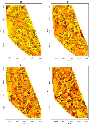
(a) (b)
(c) (d)
Figure 1. The Coefficient Process Surfaces for 1985. (a) The intercept processβ0(s); (b) the CBD distance coefficient processβ1(s); (c) the
Areal distance coefficient processβ2(s); (d) the Midway distance coefficient processβ3(s).
4. DIRECTIONAL FINITE DIFFERENCES AND DIRECTIONAL DERIVATIVE PROCESSES
We review the notions of directional finite differences and directional derivative processes for a univariate process over locations s∈ Rd. We assume that the process has mean 0 and is stationary with covariance functionC(s,s′)=K(s−s′), whereK is a valid covariance function inRd. Two frequently used isotropic forms are the power exponential class where
K()=αexp(−φν),0< ν≤2, and the Matèrn class where K()=α(φ)νKν(φ). Kν is the modified
Bessel function of orderν(Abramovitz and Stegun 1965). We use the more flexible Matèrn class here.
The univariate process{β(s):s∈Rd} is L2 (mean square) continuous ats0ifE(β(s)−β(s0))2→0 ass→s0. Under sta-tionarity, becauseE(β(s)−β(s0))2=2(K(0)−K(s−s′)), the processβ(s)is mean square continuous at allsifKis continu-ous at0. Turning to mean square differentiability,β(s)is mean square differentiable ats0if there exists a vector∇β(s0), such that for any scalarhand any unit vectoru,
β(s0+hu)=β(s0)+huT∇β(s0)+r(s0,hu), (3)
wherer(s0,hu)/h→0 in theL2sense ash→0. Withua unit vector, let
βu,h(s)=
β(s+hu)−β(s)
h (4)
be the finite difference atsin directionuat scaleh.
Next, letDuβ(s)=limh→0βu,h(s)if the limit exists.Duβ(s) is a well-defined process inRd, which we refer to as the direc-tional derivative process in the directionu. In particular, this process exists if the covariance function K is twice differen-tiable. If the unit vectorse1,e2, . . . ,edform an orthonormal ba-Hence, to study directional derivative processes in arbitrary directions, we need only work with a basis set of direc-tional derivative processes. Also from (5), it is clear that D−uβ(s)= −Duβ(s). Applying the Cauchy–Schwarz inequal-cesses at scalehin arbitrary directions, we have no reduction to a basis set.
Distribution theory for βu,h(s) and Duβ(s) is developed briefly in Appendix A. In particular, the cross-covariance functions are provided for the bivariate spatial processes (β(s), βu,h(s)) and (β(s),Duβ(s)) as well as the trivariate process (β(s),Du1β(s),Du2β(s)). It is convenient to work with the Matèrn covariance functions because the parameter v controls the smoothness of process realizations. A closed-form choice sets v=3/2, which yields once (but not twice) mean square differentiable realizations and takes the form ρ(si−s′
i, φ)=(1+φs−s′i)exp(−φs−s′i).
5. THE MODEL AND ITS DISTRIBUTION THEORY
We now return to the model in (2). Following the discussion in Section 2, we model land values on the log scale, suggest-ing that distances on the right side should go in untransformed. Therefore, apart from a first component of 1, we envision the entries inX(s)as distances fromsto various fixed externalities located at, say,s∗
l,l=2, . . . ,p. This ensures that theXl(s)are
twice differentiable, which we need later. By allowing the co-efficients to change with the location, the mean in (2) is essen-tially, as flexible as we could seek; there is no need to consider introduction of functional forms in the distances.
As noted in Section 1, McMillen (1996) also considered modeling for land values with spatially varying coefficients us-ing locally weighted regression. A brief comparison between his approach and ours might be useful. In building the model for β(s), we envision a collection ofprandom but dependent spatial surfaces, captured as a realization of a multivariate spa-tial process. McMillen hadX(s)as the argument of hisβ [in fact, the argument is a function of {X(si)}, as well]. Further-more, locally weighted regression requires an inverse distance function calculated between X(s) and each of the {X(si)}’s, yielding the distance between vectors of distances. It also re-quires an associated window width. Considering the distance betweensand thesi’s, as we do, may be more attractive. We offer full inference at each location on, for example, direc-tional gradients, the maximum gradient, and the direction of the maximum gradient. Gradients will be very difficult to study under McMillen’s model. In fact, through the posterior distri-bution, we offer an exact assessment of uncertainty associated with the coefficient vector at any location, as well as for any location on the mean surface and also for gradients of inter-est. Again, such estimation of variability will not be possible through McMillen’s model.
To provide the model specification in (2), we need to pro-pose a multivariate spatial process model forβ(s). Following Gelfand, Schmidt, Banerjee, and Sirmans (2004b), we use a lin-ear model of coregionalization (LMC) (see also Wackernagel 2003 in this regard). Specifically, we setβ(s)=Aw(s), where the components of w, the wl,l=1,2, . . . ,p, are independent
spatial processes defined onD, with mean 0 and variance 1. The wlhas an isotropic correlation function,ρ(·, φl),l=1,2, . . . ,p.
Without loss of generality, we may work with a lower triangular (Cholesky) form forA. The resultant cross-covariance function, C(β(s),β(s′)), has(l,l′)entry
Parameters in the model include the globalβvector, the lower triangularA, theφl’s, andτ2, which we collect into a vectorθ.
Now, with observations Y(si) at locations si, i=1, . . . ,n, letβ∗=(β(s1), . . . ,β(sn))T be thenp×1 column vector of a coefficient process realization. The resulting covariance matrix forβ∗is of the form
β= ˜AD˜(φ)A˜T, (6) whereA˜ =A⊗In×n andD˜(φ)is block diagonal with blocks R((φl)), where R((φl))i,i′ =(1+φlsi−si′)exp(−φlsi−
si′).
We note that marginalizing over the random effects β∗ is helpful, leaving us to run the much lower-dimensional Markov chain Monte Carlo (MCMC) algorithm forθ. Let thep×n ma-trix XT =(X(s1), . . . ,X(sn)), and let X˜ be an n×np block-diagonal matrix with its ith block entry, i=1,2, . . . ,n given byXT(si). Then the marginal likelihood becomes
L(Y;θ)∼ ||−1/2exp(−{Y−Xβ}T−1{Y−Xβ}/2), (7) whereis annp×npmatrix defined by= ˜XβX˜T+τ2I.
We assume flat normal priors for the βl’s, inverse gamma(aτ2,bτ2) for τ2, and gamma(al,bl) priors for each
of the decay parameters φl, whereas those for the entries in
the lower-triangular matrix Awere induced from an inverted Wishart prior on AAT (also see Gelfand et al. 2004a, b). We note that the joint full conditional distribution for β is mul-tivariate normal. For the rest of the parameters in θ, the full conditional distributions are nonstandard distributions and so we use a Metropolis–Hastings algorithm to sample them.
We next turn to directional derivatives associated with the model in (1). In particular, for various locations and various directions, we might seek gradients for theβl(s)’s but have pri-mary interest in gradients to theE(Y(s))surface. Note that di-rectional derivatives do not exist for theY(s)surface, because theǫ(s)surface is not even continuous, let alone differentiable.
6. INFERENCE WITH DIRECTIONAL DERIVATIVE PROCESSES
Returning to the model in (2), the mean surface EY(s)=
XT(s)β˜(s)will reveal “first-order” behavior. We can think of gradients to the mean surface as revealing “second-order” be-havior, that is, more subtle changes in theEY(s)surface. In fact, we clarify several gradients of possible interest in Section 6.1. In Section 6.2 we develop the distribution theory required to studyDuEY(s), the gradient to the mean surface at locationsin directionu. Section 6.3 provides a technical result that can be useful.
Thus, even with constant coefficients, there will be differing directional gradients at s arising strictly from the definition ofX(s). If, say,βl<0, then the component of the gradient
as-sociated withXl(s)will be most positive in the direction away
from the externality ats∗
l (u=s−s∗l) and will be 0 in the
direc-tion orthogonal to this. For a fixedu, it will be constant on an arc of fixed length abouts∗
l. In the direction away froms
∗
l, the
lth term in the sum forDuEY(s)will be constant. Hence local examination (near an externality) of gradients both on arcs and along rays should facilitate “seeing” second-order effects.
Finally, the argument for envisioning differing gradients is that in (2) there are surely omitted unobservable explanatory variables with spatial content. These effects will be reflected in the spatial error, and hence inEY(s)and thus also inDuEY(s).
6.1 Possible Gradients of Interest
Here we briefly remind the reader that several notions of gra-dients can be considered. For instance, suppose that we sim-plify to thep=2 case and considerY(s)=β0+β1X(s)+ǫ(s), whereX(s)=dist(s)= s−s∗. ThendE(Y(s))/ddist(s)=β1, the most basic gradient idea. If in this regression we transform distance, settingX(s)=g(dist(s)), then dE(Y(s))/ddist(s)=
β1g′(dist(s)).
Note that DuE(Y(s)) is entirely different. DuE(Y(s)) = β1DuX(s), but DuX(s) has nothing to do with g′(dist(s)). It is not a function of distance alone, as (8) reveals.
Now, if we replaceβ1withβ˜1(s), then we havedE(Y(s))/ dX(s)= ˜β1(s), which again has nothing to do withDuE(Y(s)). However, the mean is a function of location, not just of dis-tance froms∗. ViewingE(Y(s))as a surface, there is a gradient at each sin each directionu. We learn about rates of change in the expected land surface throughDuE(Y(s)), not through dE(Y(s))/dX(s)= ˜β1(s), the slope surface.
6.2 Further Distribution Theory
Whenp=2, consider the finite differences for the process E(Y(s))in terms of the processesβ0(s)andβ1(s). For a scale ofh, after some manipulation, the finite difference atstoward unit vectoruis given by
E(Y(s+hu))−E(Y(s))
l], the contribution of thelth term to
Du∗E(Y(s))isβ˜l(s)+Xl(s)Du∗
lβl(s). In a directionu ⊥
l ,
orthog-onal to the direction away froms∗
l,(u⊥l )T(s−s∗l)=0, and the
contribution simplifies toXl(s)Du⊥ l βl(
s).
We return to the discussion in Section 2 regarding amenities that do not change continuously. Recall that for, say, crime rate, X(s)would be a tiled surface. But then it is differentiable almost everywhere (a.e.) over the region; that is,DuX(s)exists and, in fact, equals 0 a.e. In (10), the second term on the right side for such a covariate will be 0. In the case of school quality, the contribution to (2) would take the formrβrI(s∈Br), where
Bris therth school district andIis an indicator function. So for
such a regressor, the contribution to the gradient in (10) is 0. To clarify, the foregoing regressors provide an explanation for the mean surface but will appear only partially or not at all in the gradient analysis.
From Section 4.1, the direction in which the directional derivative is maximized is
∇ET(Y(s))=
(D10E(Y(s)),D01E(Y(s)))
(D10E(Y(s)),D01E(Y(s)))
. (11)
It then follows that the directional derivative in that direction becomes
D∇E(Y(s))/∇E(Y(s))E(Y(s))
=D(1,0)E(Y(s))2+D(0,1)E(Y(s))2
1/2 . (12)
For posterior inference, we could to generate the predictive sur-face of the mean response processE(Y(s))and the associated predictive variance. For gradient behavior, we could make pos-terior predictive inference for the finite-difference process at various resolutions,h, as well as for the directional derivative process. For the latter, at locationswe need to sample the pre-dictive joint distribution of the 2p×1 vector,
Z(s)T=D(1,0)β1(s),D(0,1)β1(s), . . . ,
D(1,0)βp(s),D(0,1)βp(s)
.
Using usual composition, this requires the conditional distribu-tion ofZ(s)givenβ(si),i=1, . . . ,n, andθ. Similarly, for finite differences, for eachhand eachu, we need the 2p×1 vector
˜
Z⋆(s)T=β1(s), β1(s+hu), . . . , βp(s), βp(s+hu),
givenβ(si),i=1, . . . ,n, andθ.
Indeed, following the development in Section 4.2, both of these distributions are Gaussian with mean 0 and covariance structures given in Appendix B.
vergence theorem that (13) → 0. Hence we can conclude that DuW(s) exists and is given by DuW(s)=Dug(V(s))= g′(V(s))DuV(s).
The foregoing result can be useful in the context of land value gradients. In particular, suppose that we model Y(s), the log land value at locations. So if we considerDuE(Y(s)) we are obtaining gradients for the mean log land value sur-face. Instead, we might wish to consider gradients for the mean on a transformed scale (e.g., the original scale), that is, Dug(E(Y(s))), where, say,g(·)=exp(·). ThenDug(E(Y(s)))= g′(E(Y(s)))DuE(Y(s)). Note thatDuE(g(Y(s)))is not accessi-ble here. A new model forg(Y(s))is required; different spatial processes would be introduced. More generally, suppose that the model for W(s) is not Gaussian, but rather an exponen-tial family model as is customary in generalized linear model specification, with suitable link function g. Then E(W(s))=
g−1(V(s)Tβ(s)), and, using the result,DuE(W(s))can be ob-tained.
7. ANALYSIS OF THE OLCOTT CHICAGO DATA
We illustrate the use of our model working with theOlcott’s data for the years 1985 and 1990. For each year, we takep=4 in the model in (2), introducing distance-based regressors sim-ilar to McMillen (1996). So, in addition to an intercept sur-faceβ0(s), we bring in a coefficient surface(β1(s))for distance from the CBD, distance from Midway airport(β2(s)), and for distance from a secondary employment center (SEC), (β3(s)), resulting inβ(s)being a four-dimensional spatial process. Em-ployment centers were identified using data obtained from the Northern Illinois Planning Commission (NIPC). NIPC reports the level of employment per 1/2×1/2 square mile (a quar-ter section) for the Chicago PMSA. Areas within the Chicago area were identified as employment centers if the total employ-ment within a 1-mile radius of a quarter section was>16,000. Within the employment subcenters identified, we arbitrarily se-lected one of these employment subcenters for our analysis.
Our models were fitted using a MCMC algorithm, as outlined in Section 5. We assumed flat priors for theβl’s (the global
re-gression parameters) and a gammaG(.0001, .0001)(mean 1.0; variance 1.0E+8) prior for the precision 1/τ2. For the parame-ters in the four-dimensional spatial process, we assumed weakly informative gamma priors for the four correlation decay pa-rameters (scaled to have a mean range of about half of the maximum distance), whereas an inverted-Wishart IW(4, .01I4) prior (with 4 degrees of freedom, and diagonal means=100) forAATinduces the prior onA. Convergence was diagnosed by monitoring the mixing of two parallel chains with overdispersed starting values. With Gaussian likelihoods and weakly informa-tive priors, convergence was diagnosed within 2,000 iterations, with a further 1,000 iterations retained from each chain as pos-terior samples.
In the interest of simple model comparison, we also fitted a version of (2) with only a spatially varying intercept (i.e., a usual spatial random effect), that is, with constant coefficients for the distance-based regressors. We used the posterior pre-dictive model selection criterion of Gelfand and Ghosh (1998). LettingGdenote the goodness-of-fit term,Pdenote the penalty
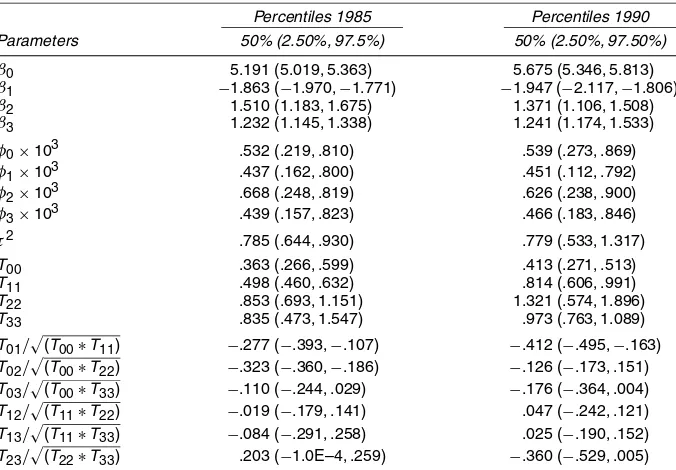
Table 1. Posterior Estimates of Model Parameters for the Olcott Data, 1985 and 1990
Percentiles 1985 Percentiles 1990
Parameters 50% (2.50%, 97.5%) 50% (2.50%, 97.50%)
β0 5.191 (5.019, 5.363) 5.675 (5.346, 5.813) β1 −1.863 (−1.970,−1.771) −1.947 (−2.117,−1.806) β2 1.510 (1.183, 1.675) 1.371 (1.106, 1.508) β3 1.232 (1.145, 1.338) 1.241 (1.174, 1.533) φ0×103 .532 (.219, .810) .539 (.273, .869)
T22 .853 (.693, 1.151) 1.321 (.574, 1.896)
T33 .835 (.473, 1.547) .973 (.763, 1.089)
term, andDdenote the criterion value, for 1985, for the sim-pler model G=.202, P=.501, and D=.703, whereas for the spatially varying coefficient model, G=.168, P=.513, andD=.681. For 1990, we obtainG=.189, P=.511, and D=.700 withG=.157,P=.521, andD=.678. So the full model is preferred, and hence we present posterior inference under this model including the gradient analysis.
The posterior inferences for 1985 and 1990 are summarized in Table 1. The intercept for 1990 is slightly greater than that for 1985, indicating increased land value over time. The four global regression parameters, for both years, reveal a negative impact on land value for the distance from the CBD (land value decreases for locations distant from the CBD) and an oppo-site effect (land value increasing with distance) for the other two distances. The result related to Midway is not surprising when one considers that the sample is dominated by residential land values. Close proximity to areas of congestions and sig-nificant noise, such as Midway, leads to lower land values. At first, the positive effect on land values at greater distances from SEC seems counterintuitive until one considers the location of this employment subcenter. Its location is to the southeast of the CBD and approximately 1.6 km to the west of the shore of Lake Michigan. The positive parameter could reflect the proximity to the CBD, but as our analysis shows, it more likely is attributed to a lake effect found in this region.
Also shown are estimates of the correlation decay para-meters, the measurement error τ2, and the spatial variance– covariance parameters as appearing in the matrix T(with the covariances converted to correlations). The relatively large con-tributions ofT00 throughT33 toward the variability justifies a rather rich spatial model for the data. Also, the tendency toward negative correlation between the intercept and the regression parameters (with some being significantly so) is expected.
Turning to Figures 1 and 2, we plot the coefficient process surfaces for 1985 and 1990. These are image plots with over-laid contour lines indicating the levels. The rather rich distribu-tion of contours seem to justify our use of the spatially varying coefficients.
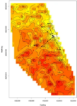
Figures 3 and 4 plot the posterior means of the mean surfaces for 1985 and 1990. In general, we find from the mean land value price surface that the surface’s maximum value corresponds to the location of the CBD and that land prices fall as one moves further from the lake in both time periods. However, the results do not support the idea of a constant gradient over the entire ur-ban area in either time period. In fact, the gradient’s magnitude not only varies with location, but also depends on the direction from the center of the city for which it is evaluated. The gra-dient is also found to be steepest close to the CBD and then flattens in all directions as distance increases.
Both mean surfaces suggest several directions to examine. Note that the putative location of the CBD is at the intersection of the 447902.14038 Easting and 4636874.42216367 Northing near Lake Michigan and is at the conjunction of the four rays in each figure. The four rays denote the four directions in which we travel to understand gradient behavior. These directions are indicated in the figures as NLk (Northern Lake vicinity), NW (Northwest of the CBD), SW (Southwest of the CBD), and SLk (Southern Lake vicinity). Tables 2 and 3 examine several points at different distances (indicated as .5, 1.5, 3.0, and 6.0) from the CBD in kilometer units. For each ray, two fundamental direc-tional gradients are evaluated: (a) movingawayfrom the CBD alongthe ray, and (b) the directionnormalor orthogonal to the ray. Note that movingtowardthe CBDalonga ray would be the negative of that evaluated in (a).
A closer look at Tables 2 and 3 for the directional gradi-ents evaluated at points along the different rays reveals that a strong gradient exists in all directions from the CBD. This gra-dient is steepest close to the CBD and tends to diminish as dis-tance increases. This flattening seems to be more abrupt for the 1990 data than for 1985. Indeed, if we imagine an arc pass-ing through the .5 km points, then the directional gradients are significantly negative and quite similar in magnitude. But this slope steadily decreases in significance when the arc is extended to pass through the 1.5-, 3.0-, and 6.0-km points. For example,
(a) (b)
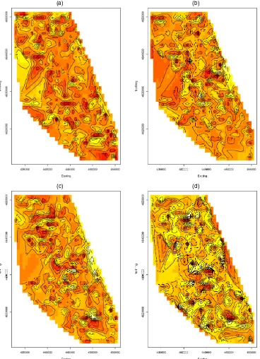
(c) (d)
Figure 2. The Coefficient Process Surfaces for 1990. (a) The intercept processβ0(s); (b) the CBD distance coefficient processβ1(s); (c) the
Areal distance coefficient processβ2(s); (d) the Midway distance coefficient processβ3(s).
for the 1985 data, significant gradients along the NW and SW rays are seen up to 3 km, whereas for the 1990 data they are seen only until the 1.5-km points. No significant gradients are seen in the orthogonal directions to the NW and SW rays.
Traveling north and south of the CBD along the rays NLk and SLk, we come across a more interesting phenomenon. As before, the diminishing impact of the CBD is manifested with gradients along these rays (away from the CBD) becoming less pronounced. For the northern lake region, they are significant up to the 3-km point (barely) for 1985 and the .5-km point for 1990, whereas for southern region they are significant up to the 1.5-km point for 1985 and the .5-km point for 1990. For the
or-thogonal direction, however, the gradients become significant for the 3- and 6-km points for 1985 and are quicker for 1990, when they are significant immediately after the .5-km point. Apparently, beyond a certain distance from the CBD, proxim-ity to Lake Michigan becomes a prominent determinant for land value gradients.
To further illuminate the inferential ability of our approach, two locations anticipated to reveal differential gradient beha-vior—an SEC and a secondary population center (SPC)—were chosen employment and population centers are important parts of the urban geography. The agglomeration economies associ-ated with employment centers, as well as the clustering of
Figure 3. Posterior Mean Surface and Locations for Directional Gra-dient Analysis in the 1985 Olcott Data. See text for details.
dividuals to benefit from neighborhood amenities, should lead to interesting land value gradient patterns. The SEC is lo-cated at 450040.902 Easting, 4626786.843 Northing and was used in part of the foregoing analysis. The SPC is located at 441062.526 Easting, 4633147.015 Northing. Both are labeled in Figures 3 and 4. For each point, we obtained posterior distri-butions of the angle of the maximal gradient relative to the line
Figure 4. Posterior Mean Surface and Locations for Directional Gra-dient Analysis in the 1990 Olcott Data. See text for details.
from the point to the CBD for both 1985 and 1990, as well as the posterior distribution of the difference between the maximal gradient and the gradient in the direction away from the CBD. These plots are shown in Figures 5 and 6.
Because these two points are rather far from the CBD, simple contour analysis or other descriptive methods are inadequate for formal evaluation of the foregoing geometric quantities.
How-Table 2. Directional Derivative Gradients at Different Directions Related to 1985 Data
Away from CBD Orthogonal to direction away from CBD
Points Percentiles 50% (2.5%, 97.5%) Percentiles 50% (2.5%, 97.50%)
NW.5 −2.761 (−4.004,−1.512) −.264 (−1.203, 1.479) NW1.5 −2.047 (−3.243,−.858) .047 (−1.091, 1.152) NW3.0 −1.492 (−2.782,−.285) .151 (−1.277, 1.367) NW6.0 −.041 (−1.564, 1.482) −.621 (−2.038, .583) SW.5 −2.727 (−3.926,−1.104) −.142 (−1.343, 1.205) SW1.5 −2.014 (−3.253,−.737) .045 (−1.152, .929) SW3.0 −1.210 (−2.382,−.037) −.044 (−1.169, 1.001) SW6.0 −.005 (−1.459, 1.450) −.101 (−1.09, .991) NLk.5 −2.596 (−4.001,−1.262) −.107 (−1.129, 1.021) NLk1.5 −1.481 (−2.801,−.202) −.358 (−1.948, 1.036) NLk3.0 −.947 (−1.959,−.007) −2.095 (−3.036,−1.031) NLk6.0 −.922 (−1.883, .306) −1.434 (−2.626,−.549) SLk.5 −2.653 (−3.851,−1.474) .118 (−1.026, 1.002) SLk1.5 −1.880 (−2.793,−.843) .149 (−.982, 1.223) SLk3.0 −1.334 (−2.492, .032) −1.062 (−2.291,−.021) SLk6.0 −.898 (−1.994, .195) −2.153 (−3.278,−1.087)
Table 3. Directional Derivative Gradients at Different Directions Related to 1990 Data
Away from CBD Orthogonal to direction away from CBD
Points Percentiles 50% (2.5%, 97.50%) Percentiles 50% (2.5%, 97.50%)
NW.5 −2.457 (−4.166,−.776) .255 (−1.296, 1.670) NW1.5 −2.165 (−3.818,−.094) .110 (−1.386, 1.452) NW3.0 −1.366 (−3.179, .440) .135 (−1.387, 1.539) NW6.0 −1.221 (−3.008, .292) .208 (−1.284, 1.510) SW.5 −2.307 (−3.851,−.796) −.183 (−1.584, 1.166) SW1.5 −2.078 (−3.536,−.381) −.081 (−1.592, 1.663) SW3.0 −.492 (−1.939, .836) 1.033 (−.492, 2.311) SW6.0 −1.217 (−2.836, .063) .502 (−1.106, 1.996) NLk.5 −2.212 (−3.974,−.587) .324 (−1.305, 2.073) NLk1.5 .088 (−1.906, 1.603) −1.333 (−3.046, .560) NLk3.0 .034 (−1.415, 1.280) −.967 (−2.738, .802) NLk6.0 −1.044 (−2.371, .723) −1.057 (−2.502, .302) SLk.5 −2.493 (−4.197,−.868) .036 (−1.631, 1.653) SLk1.5 −.170 (−1.951, 1.025) −2.248 (−4.212,−.524) SLk3.0 −.054 (−1.467, 1.657) −2.586 (−3.902,−.633) SLk6.0 −.150 (−1.632, 1.332) −2.084 (−3.665,−.754)
ever, using our sampling-based methods, we find that SPC has a maximal gradient direction not significantly different from the direction away from the CBD (contains 0). On the other hand, SEC, being in the southeast along the lake has a much more sig-nificant difference between the maximal gradient direction and the direction from the CBD for both years. In support, Tables 2 and 3 show that in both 1985 and 1990, the gradient quickly becomes flat along a ray moving south along the lake away from the CBD, whereas the gradient orthogonal to this
direc-tion stays significant. Thus the gradient is larger in a westerly direction (90◦), that is, perpendicular to the lake. However, Fig-ure 6 shows that the direction of maximal gradient is expected to be roughly southwest (45◦) from the lake.
8. DISCUSSION AND EXTENSIONS
We have developed a general theoretical approach, includ-ing full distribution theory, to examine gradients associated
(a) (b)
(c) (d)
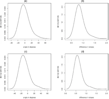
Figure 5. Density of Angle Between Ray of Maximum Gradient and CBD in Degrees and the Absolute Difference Between Values of Maximal Gradient and Directional Gradient From CBD for SPC in the Olcott Data. (a) and (b) 1985; (c) and (d) 1990. See text for details.
(a) (b)
(c) (d)
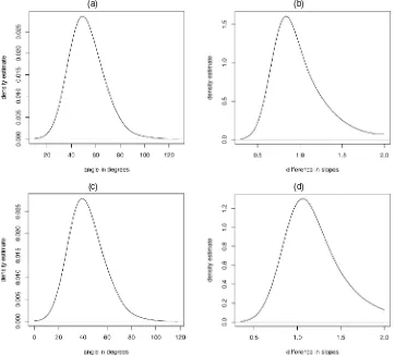
Figure 6. Density of Angle Between Ray of Maximum Gradient and CBD in Degrees and the Absolute Difference Between Values of Maximal Gradient and Directional Gradient From CBD for SEC. (a) and (b) 1985; (c) and (d) 1990. See text for details.
with spatially varying coefficient models. The theory was built through dependent spatial coefficient and intercept surfaces and yields a resulting mean surface. Gradients at arbitrary locations in arbitrary directions can be studied for each of these surfaces. Also, at a point, for these surfaces the distribution of the direc-tion of maximum gradient and the magnitude of the maximum gradient can be obtained. Working within a Bayesian frame-work allows this full range of inference. Our motivation was to study land value gradients, but other potential applications where gradient analysis of the mean surface would be of inter-est include weather and pollution data modeling.
We have focused on explaining land value as a function of distance from the CBD as well as from other “externalities.” Using various distances as explanatory variables, when applied to an urban area like Chicago, we have shown that the simple economic theory asserting exponential decay in distance is not valid. In fact, we have provided a collection of tables and fig-ures that reveal the more subtle nature of expected land value surfaces. At a global level, we see departure from the theoret-ical suggestion, but at a local (point) level, we see even more subtle departure.
Some cities are known to be multicentric (Los Angeles, for example). The distance-based regressors model of the previ-ous section is again appropriate here. Furthermore, we have clarified how non–distance-based regressors and, more gener-ally, regressors that need not be continuous can be introduced, noting that suitable spatially varying coefficient models can
still be fitted. In this regard, we have indicated their effect on the gradient analysis. Finally, the Olcott data are available for 13 time points, roughly equally spaced. Space–time modeling forY(s,t), withtindicating the time point, extending (16) can be developed. This problem will be pursued in future work.
APPENDIX A: DISTRIBUTION THEORY
Here, continuing from Section 4, we provide the basic dis-tribution theory for directional finite difference processes and directional derivative processes. IfE(β(s))=0 for alls∈Rd,
then clearlyE(βu,h(s))=0 andE(Duβ(s))=0. LetC(uh)(s,s′) andCu(s,s′)denote the covariance functions associated with the process βu,h(s) and Duβ(s). If =s−s′ and β(s) is (weakly) stationary, then we immediately have
C(uh)(s,s′)=
(2K()−K(+hu)−K(−hu))
h2 , (A.1)
where var(βu,h(s))=2(K(0)−K(hu))/h2. Ifβ(s)is isotropic,
then we obtain
C(uh)(s,s′)=
(2K()−K(+hu)−K(−hu))
h2 .
(A.2) Expression (A.2) shows that even ifβ(s)is isotropic, βu,h(s)
is only stationary. In addition, var(βu,h(s))=2(K(0)−K(h))/
h2=γ (h)/h2, whereγ (h)is the familiar variogram of theβ(s) process (Cressie 1993).
Similarly, ifβ(s)is stationary, then we may show that if all second-order partial and mixed derivatives ofK exist and are continuous, then the limit of (A.1) ash→0 is
For β(s) stationary, we can also calculate cov(β(s), βu,h(s′))=(K(−hu)−K())/h, from which cov(β(s), rectional derivative process ensures the existence ofDuK(0).
Under isotropy, cov(β(s), βu,h(s′)) = (K( − hu) − a valid cross-covariance matrix in Rd. But since this is true everyh, lettingh→0
is a valid cross-covariance matrix inRd. In fact,Vuis the cross-covariance matrix for the bivariate processZu(s)= β(
s)
Duβ(s)
. If, in addition, we assume thatβ(s)is a stationary Gaussian process, then it is clear, again by linearity, thatZhu(s)is a sta-tionary bivariate Gaussian process. But then, by a standard limiting moment-generating function argument,Zu(s)is a sta-tionary bivariate Gaussian process, and thus Duβ(s)is a sta-tionary bivariate Gaussian process.
Suppose that we consider a pair of directions with associated vectors u1 andu2. With β(s) a stationary Gaussian process,
we can argue as before that if Zu1,u2,h(s)=
Banerjee et al. (2003). Passing to the limit ash→0, we obtain the valid cross-covariance function for Zu1,u2(s)=
Here we provide the covariance structures corresponding to Z⋆(s)and Z˜⋆(s) from Section 6.2. LetK
1 denote the cor-relation function of the processw1(s)andK2 denote the cor-relation function of the process w2(s). Let 1 and2be the Hessian matrices corresponding to w1(s) and w2(s). Apply-ing the results from Banerjee et al. (2003), we have(l)i,i′=
δ2
δiδi′Kl(),l=1,2.
We know that it is sufficient to derive the directional deriv-ative processes in terms of the two orthonormal vectors of di-rectionse1=(0,1)ande2=(1,0)inR2. From Banerjee et al. (2003), we get the following results related to the covariance structure of Z⋆(s): cov(D
[Received January 2003. Revised June 2005.]
REFERENCES
Abramowitz, M., and Stegun, I. A. (1965),Handbook of Mathematical Func-tions With Formulas, Graphs and Mathematical Tables, New York: Dover. Alperovich, G., and Deutsch, J. (2002), “An Application of a Switching
Regimes Regression to the Study of Urban Structure,”Papers in Regional Science, 81, 83–98.
Banerjee, S., Gelfand, A. E., and Sirmans, C. F. (2003), “Directional Rates of Change Under Spatial Process Models,”Journal of the American Statistical Association, 98, 946–954.
Black, S. (1999), “Do Better Schools Matter? Parental Valuation of Elementary School Education,”Quarterly Journal of Economics, 114, 577–600. Cheshire, P., and Sheppard, S. (1995), “On the Price of Land and the Value of
Amenities,”Economica, 246, 247–267.
Cleveland, W. S., and Devlin, S. J. (1988), “Locally Weighted Regression: An Approach to Regression Analysis by Local Fitting,”Journal of the American Statistical Association, 83, 596–610.
Colwell, P. F., and Dilmore, G. (1999), “Who Was First? An Examination of an Early Hedonic Study,”Land Economics, 75, 620–626.
Colwell, P. F., and Munneke, H. J. (1997), “The Structure of Urban Land Prices,”Journal of Urban Economics, 41, 321–336.
(2004), “Directional Land Value Gradients,” unpublished manuscript, The University of Georgia.
Cressie, N. A. C. (1993),Statistics for Spatial Data, New York: Wiley. Epple, D., and Seig, H. (1999), “Estimating Equilibrium Models of Local
Ju-risdictions,”Journal of Political Economy, 107, 645–681.
Ferreyra, M. (2003), “Estimating the Effects of Private School Vouchers in Multi-District Economies,” unpublished manuscript, Carnegie Mellow Uni-versity.
Gelfand, A. E., Ecker, M. D., Knight, J. R., and Sirmans, C. F. (2004a), “The Dynamics of Location in Home Price,”Journal of Real Estate and Financial Economics, 29, 149–166.
Gelfand, A. E., and Ghosh, S. K. (1998), “Model Choice: A Minimum Posterior Predictive Loss Approach,”Biometrika, 85, 1–11.
Gelfand, A. E., Kim, H.-J., Sirmans, C. F., and Banerjee, S. K. (2003), “Spa-tial Modeling With Spa“Spa-tially Varying Coefficient Processes,”Journal of the American Statistical Association, 98, 387–396.
Gelfand, A. E., Schmidt, A. M., Banerjee, S., and Sirmans, C. F. (2004b), “Non-stationary Multivariate Modeling Through Spatially Varying Coregionaliza-tion,”Test, 13, 1–50.
Haas, G. (1922), “Scales Prices as a Basis for Farm Land Appraisal,” Technical Bulletin 9, The University of Minnesota Agricultural Experiment Station, St. Paul.
Janssen, C., and Soderberg, B. (2001), “Estimating Density Gradients for Apartment Properties,”Urban Studies, 31, 61–80.
Kau, J. B., and Sirmans, C. F. (1979), “Urban Land Value Functions and the Price Elasticity of Demand for Housing,”Journal of Urban Economics, 6, 112–121.
Kent, J. T. (1989), “Continuity Properties for Random Fields,”The Annals of Probability, 17, 1432–1440.
Luo, Z., and Wahba, G. (1998), “Spatio-Temporal Analogues of Temperature Using Smoothing Spline ANOVA,”Journal of Climatology, 11, 18–28. Matèrn, B. (1986),Spatial Variation(2nd ed.), Berlin: Springer-Verlag. McDonald, J. F., and Bowman, H. W. (1979), “Land Value Functions: A
Reeval-uation,”Journal of Urban Economics, 6, 25–41.
McMillen, D. P. (1996), “One Hundred Fifty Years of Land Values in Chicago: A Nonparametric Approach,”Journal of Urban Economics, 40, 100–124. McMillen, D. P., and McDonald, J. F. (1989), “Selectivity in Urban Land Value
Functions,”Land Economics, 65, 34251.
Mills, E. S. (1971), “The Value of Urban Land,” inThe Quality of the Ur-ban Environment, ed. H. Perloff, Washington, DC: Resources for the Future, pp. 231–253.
(1972),Studies in the Structure of the Urban Economy, Baltimore: Johns Hopkins Press, Resources for the Future, pp. 96–127.
Muth, R. F. (1969),Cities and Housing, Chicago: University of Chicago Press. Pace, R. K., Barry, R., and Sirmans, C. F. (1998), “Spatial Statistics and Real
Estate,”The Journal of Real Estate Finance and Economics, 17, 5–13. Schoenberg, I. J. (1938), “Metric Spaces and Completely Monotone Functions,”
Annals of Mathematics, 39, 811–841.
Sieg, H., Smith, V. K., Banzhaf, S., and Walsh, R. (2004), “Estimating the Equi-librium Benefits of Large Changes in Spatially Delineated Public Goods,”
International Economic Review, 45, 1047–1077.
Stein, M. L. (1999),Interpolation of Spatial Data: Some Theory for Kriging, New York: Springer-Verlag.
Wackernagel, H. (2003),Multivariate Geostatistics: An Introduction With Ap-plications(3rd ed.), Berlin: Springer-Verlag.
Wilhelmsson, M. (2002), “Spatial Models in Real Estate Economics,”Housing, Theory and Society, 19, 92–101.