Manajemen | Fakultas Ekonomi Universitas Maritim Raja Ali Haji 08832320309598624

(1)

Full Terms & Conditions of access and use can be found at

http://www.tandfonline.com/action/journalInformation?journalCode=vjeb20

Download by: [Universitas Maritim Raja Ali Haji] Date: 12 January 2016, At: 23:58

Journal of Education for Business

ISSN: 0883-2323 (Print) 1940-3356 (Online) Journal homepage: http://www.tandfonline.com/loi/vjeb20

An Algorithm for Using Excel Solver© for the

Traveling Salesman Problem

Mike C. Patterson & Bob Harmel

To cite this article: Mike C. Patterson & Bob Harmel (2003) An Algorithm for Using Excel Solver© for the Traveling Salesman Problem, Journal of Education for Business, 78:6, 341-346, DOI: 10.1080/08832320309598624

To link to this article: http://dx.doi.org/10.1080/08832320309598624

Published online: 31 Mar 2010.

Submit your article to this journal

Article views: 124

(2)

An Algorithm for Using

Excel Solver@ for the Traveling

Salesman Problem

MIKE C. PATTERSON

BOB HARMEL

zyxwvutsrqponmlkjihgfedcbaZYXWVUTSRQPONMLKJIHGFEDCBA

Midwestern State University

Wichita Falls, Texas

or years, the amount of time

F

required to formulate and solve linear programming problems has been a significant hurdle for researchers, business educators, and business com- munity practitioners. Linear programming is a powerful tool, but the lack of readily available and efficient solution algorithms has limited its practicality in many business applications

Our purpose in this article is to dem- onstrate the efficiency of a problem- solving algorithm that uses the readily available spreadsheet add-in Microsoft Excel Solver@. We selected Solver because it is widely available and has a marginal software cost of zero. It comes with the standard Microsoft Excel package. If a user has Microsoft

Office

zyxwvutsrqponmlkjihgfedcbaZYXWVUTSRQPONMLKJIHGFEDCBA

2000, he or she has Solver,

which can be applied very effectively to small and medium-sized linear programming problems. For larger problems, other optimization software add- ins such as Riskoptimizer and Premium Solver Platform may be pur- chased from Microsoft at a higher cost. The Traveling Salesman Problem (TSP) has challenged operations research enthusiasts for decades. One of the earliest articles published on the problem was “On the Hamiltonian Game (a traveling-salesman problem),” by J. B. Robinson (1949). Six years later, Dantzig, Fulkerson, and Johnson

ABSTRACT. The Traveling Sales- man Problem (TSP), well known to operations research enthusiasts, is one of the most challenging combinatorial optimization problems. In this article, the authors present one approach to solving a classic TSP through a special purpose linear programming model, zero-one programming, and Microsoft Excel@Solver.

(1954) published one of the best known TSP papers, “Solution of a Large-Scale Traveling-Salesman Problem.” That article documented the use of a special application of linear programming for solving a 49-city problem.

The objective of the TSP problem can be defined as follows:

Minimize the total distance of a tour through a given number of locations, beginning and ending the tour in the same location and entering and leaving each location once.

Over the past 50 years, mathemati- cians have studied the TSP problem extensively. One of the best known TSP projects is supported by Rice University, Rice’s Computer and Information Tech- nology Institute; the Center for Research on Parallel Computation; Digital Equip- ment Corporation; and the Keck Foun- dation. Two, of the better known TSP

Web sites are <http://www.iwr.unihei

zyxwvutsrqponmlkjihgfedcbaZYXWVUTSRQPONMLKJIHGFEDCBA

delberg.de/iwr/comopt/sofware/TSPLIB

95/> and <http://riceinfo.rice.edu/proj ects/reno/rn/l9980625/tsp.html>.

Linear programming, one of the most widely used operations research tools, is of interest to operations researchers, business college educators, and business practitioners. Zero- one programming, a special form of linear programming, allows variables to take on only values of zero or one. Solver, the software add-in tool for Microsoft Excelo, also has been the model for special applications of linear programming such as the assignment (Patterson & Harmel, 2001) and transportation problems (Patterson & Harmel, 2002). In this article, we present an algorithm for using linear programming/zero-one programming and Solver in the solution of a seven-city traveling salesman problem.

Traveling Salesman Problem

zyxwvutsrqponmlkjihgfedcbaZYXWVUTSRQPONMLKJIHGFEDCBA

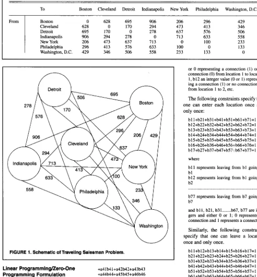
A TSP is usually presented as a table.

In Table 1, we summarize the pertinent data for our TSP. As stated previously,

the objective is to find the route that minimizes the total distance traveled and has the traveler begin in one city (e.g., Boston), enter and exit each city once, and end the trip in the beginning city (Boston). The complexity of this problem is perhaps better illustrated through a diagram (see Figure 1 for a

schematic of the problem).

zyxwvutsrqponmlkjihgfedcbaZYXWVUTSRQPONMLKJIHGFEDCBA

July/August 2003 341

(3)

TABLE 1. Road Mileage Dlstances Between Cities

zyxwvutsrqponmlkjihgfedcbaZYXWVUTSRQPONMLKJIHGFEDCBA

From

To Boston

~~ ~~

Boston Cleveland Detroit Indianapolis

New

York

Philadelphia Washington, D.C.

0

628 695 906 206 296 429

Cleveland Detroit Indianapolis New York Philadelphia Washington, D.C. 628 695 906 206 296 429

0 170 294 473 413 346

170 0 278 637 576

506

294 278 0 713 633 558 473 637 713 0 100 233 413 576 633 100 0 133

346 506 558 233 133 0

[image:3.612.42.551.67.615.2]

u

FIGURE 1. Schematic of Traveling Salesman Problem.

Linear ProgrammingRero-One Programming Formulation

tive function for this problem:

The following represents the objec-

Minimize:

allbll+a12b12+a13b13 +a14b14+al5b 15+a 16b 16 +a17b17+a2 1 b2 1 +a22b22 +a23b23+a24b24+a25b25 +a26b26+a27b27+a31b31 +a32b32+a33b33+a34b34 +a35b35+a36b36+a37b37

+a41 b41+a42b42+a43b43 +a44b44+a45b45+a46b46 +a47b47+aSlbSl+a52b52 +a53b53+a54b54+a55b55 +a56b56+a57b57+a61b61 +a62b62+a63b63+a64b64 +a65b65+a66b66+a67b67 +a71b7 l+a72b72+a73b73 +a74b74+a75b75+a76b76 +a77b77

where a l l = value from distance table (Table 1) from row 1 column 1, a12 = distance from row 1 column 2, etc.; and where b l l = an integer value of either 1

or 0 representing a connection (1) or no connection (0) from location 1 to location 1, b12 an integer value (0 or 1) representing a connection (1) or no connection (0)

from location 1 to 2, etc.

The following constraints specify that one can enter each location once and only once:

bll+b21+b31+b41+b51+b61+b71=1 b12+b22+b32+b42+b52+b62+b72=1 b13+b23+b33+b43+b53+b63+b73=1 b14+b24+b34+b44+b54+b64+b74=1 blS+b25+b35+b45+b55+b65+b75=1 b16+b26+b36+b46+b56+b66+b76=1 b17+b27+b37+b47+b57:.b67+b77=1

where

bl 1 represents leaving from b 1 going to bl

b12 represents leaving from bl going to b2

b77 represents leaving from b7 going to b7

and b l l , b21, b31

...

b67, b77 are integers and either 0 or 1; 0 represents no connection and 1 represents a connection.

Similarly, the following constraints specify that one can leave a location once and only once.

bll+b12+b13+b14+b15+bl6+b17=1 b21+b22+b23+b24+b25+b26+b27=1 b31+b32+b33+b34+b35+b36+b37=1 b41+b42+b43+b44+b45+b46+b47=1 b51+b52+b53+b54+b55+b56+b57=1 b61+b62+b63+b64+b65+b66+b67=1 b71+b72+b73+b74+b75+b76+b77=1

The following constraints define the bmn variables as either 0 or 1 :

bll>=Obll<=l b12>=0b12<=1 b13>=0b13<=1 b76>=0b76<=1 b77>=0b77<=1

342

zyxwvutsrqponmlkjihgfedcbaZYXWVUTSRQPONMLKJIHGFEDCBA

Journal

of Education for Business

(4)

The following constraints do not allow

one to enter and leave the same city:

bll=Ob22=0 b33=0b44=0 b55=0b66=0 b77=0

The final constraints are formulated for elimination of the initial subtours. Because the tour must begin and end in the same city, these subtours must be eliminated. The initial subtour constraints are the following:

b12+b21<=lb34+b43<=1 b13+b31<=lb35+b53<=1 b14+b41<=lb36+b63<=1 b15+b51<=lb37+b73<=1 b16+b61<=lb45+b54<=1 b17+b71<=0b46+b64<=1 b23+b32<=lb47+b74<=1 b24+b42<=lb56+b65<=1 b25+b52<=lb57+b75<=1 b26+b62<=lb67+b76<=1 b27+b72<=1

These constraints prevent the model from suggesting a trip from Boston to Cleveland to Boston, from Boston to Detroit to Detroit, and so forth.

Other subtours are possible when the solver uses linear (zero-one) programming for traveling salesman problems. Identifying all of the possible subtours is not necessary in the initial formulation. We identify and discuss these subtours.

C

From

zyxwvutsrqponmlkjihgfedcbaZYXWVUTSRQPONMLKJIHGFEDCBA

Solver Formulation and Solution

The Solver add-in tool is located under the Tools icon in Excelo. If it is not available, it will need to be added from the custom install program fpr Excelo. Solver was developed for Microsoft by Frontline Systems Inc., which also developed similar add-ins for Lotus 123 and QuatroPro. The Web page maintained by Frontline (http:l/ www.solver.com/) provides useful information regarding the use of optimization and the availability of more powerful versions of Solver.

To solve TSPs, one can use Microsoft Excel Solvero and follow the linear programming formulation above.

Step 1. Define two spreadsheets. These spreadsheets should be based on the typical traveling salesman problem as defined in Table 1. The first spreadsheet should contain the distance frondto each of the cities in the problem. The second spreadsheet should duplicate the headings from the first matrix and should contain zeros in the body of the spreadsheet, indicating, as discussed above, no connection. We show the spreadsheets in Table 2.

Step 2. Define row and column totals for spreadsheet 2. The following is a partial listing of the definitions:

D E F

zyxwvutsrqponmlkjihgfedcbaZYXWVUTSRQPONMLKJIHGFEDCBA

G H I

J K To Boston Cleveland Detroit Indianapolis New York Philadelphia Washington, D.C.

Boston 0 628 695 906 206 296 429

Cleveland 628 0 170 294 473 413 346

Detroit 695 170 0 278 637 576 506

Indianapolis 906 294 278 0 713 633

558

New York 206 473 637 713 0 100 233

Philadelphia 296 413 576 633 100 0 133

Washington, D.C. 429 346 506 558 233 133 0

To Boston Cleveland Detroit Indianapolis New York Philadelphia Washington, D.C. CellFormula

E19=SUM(E12..E18) F19=SUM(F12..FI 8)

G19=SUM(G12..G 18) L17=SUM(E17..K17) L18=SUM(E18..KI 8)

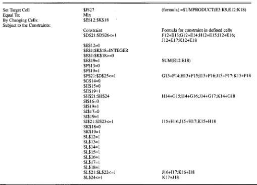
Step 3. Define the payoff cell. In this example, the payoff cell is defined in 527. The payoff is the sum of the prod- uct of spreadsheet (matrix) 1 times spreadsheet 2. The Excel@ formula to calculate the payoff is: =SUMPROD UCT(E3:K9,E 12:K 18).

Step

4.

Define the objective. This is executed by choosing “Tools/Solver,” “Set Target Cell.” The cell in this example is $J$27.

Step 5 . Define the cells to change. This is done by identifying the cells in “By Changing Cells.” The cells in this example are the zero cells in spreadsheet 2: $E$12:$K$18.

Step

zyxwvutsrqponmlkjihgfedcbaZYXWVUTSRQPONMLKJIHGFEDCBA

6 . Define the constraints. This is

done in the Solver section “Subject to Constraints.” When defining the constraints, one should refer to the linear programming section. We show the complete Solver parameters in Table 3.

Step 7. Select the appropriate options for Solver. Select “Assume Linear Model.”

From Boston 0 0 0 0 0 0 Cleveland 0 0 0 0 0 0 Detroit 0 0 0 0 0 0 Indianapolis 0 0 0 0 0 0

New York 0 0 0 0 0 0 Philadelphia 0 0 0 0 0 0

Washington, D.C. 0 0 0

zyxwvutsrqponmlkjihgfedcbaZYXWVUTSRQPONMLKJIHGFEDCBA

0 0 0

July/August 2003 343

(5)

TABLE 3. Solver Formulation of Traveling Salesman Problem

zyxwvutsrqponmlkjihgfedcbaZYXWVUTSRQPONMLKJIHGFEDCBA

Set Target Cell

Equal To:

By Changing Cells: Subject to the Constraints:

$J$27 Min

$E$12:$K$18 Constraint $D$21:$D$26<=1 $E$12=0

$E$I:$K$l8=INTEGER $E$ 1 :$K$18>=0 $E$19=1 $F$13=0 $F$19= 1

$F$21 :$D$25<=1 $G$14=0 $H$15=0 $H$19=1 $H$21:$H$24 $1$16=0 $1$19= 1 $J$17=0

$J$19= 1

$J$21 :$J$23<=1 $K$18=0 $K$l9=1 $L$12=1 $L$13=1 $L$14=1 $L$15=1 $L$16=1 $L$17=1 $L$18=1 $L$2 1 :$L$22<= 1 $L$24<= 1

(formula)

=SUMPRODUCT(E3:K9,E12:K18)

Formula for constraint in defined cells F12+E13;G 12+E14;H 12+E 15;112+E 16; J12+E17;K12+E18

H 14+G 15;114+G 1 6 3 14+G 17;K14+G 1 8 115+H16;JI 5+H17;K15+H 18

J 16+117;K16+118 K17+J18 TABLE 4. Initial Solution to Traveling Salesman Problem

To Boston Cleveland Detroit Indianapolis New York Philadelphia Washington, D.C. From Boston 0 0 0

Cleveland 0 0 1 Detroit 0 0 0

New York

zyxwvutsrqponmlkjihgfedcbaZYXWVUTSRQPONMLKJIHGFEDCBA

1 0 0 Indianapolis 0 I 0

Philadelphia 0 0 0 Washington, D.C. 0 0 0

1 1 I

0 1

0 1 0 1 1 1

0 1

1

TABLE 5. Subtour Constraints

J12+117+K16+EI 8<=3 Boston-Philadelphia-New York-Washington, D.C.-Boston

112+K16+J18+E17<=3 Boston-New York-Washington, D.C.-Philadelphia-Boston

112+J16+K17+EI 8<=3 Boston-New York-Philadelphia-Washington, D.C.-Boston

K 12+J 18+I 17+E 16<=3 Boston-Washington, D.C.-Philadelphia-New York-Boston

K12+I 18+516+E17<=3 Boston-Washington, D.C.-New York-Philadelphia-Boston . .

344

zyxwvutsrqponmlkjihgfedcbaZYXWVUTSRQPONMLKJIHGFEDCBA

Journal of Education for

Business [image:5.612.54.563.66.433.2]

(6)

Step 8. Format the cells D12:J18 to be numbers with 0 decimal points. Extensive testing with Solver indicates that even if the values are defined as integers, Solver will frequently provide very small nonin- teger values such as 2.34444E-14. To force the spreadsheet to provide only 0 or 1 in the second spreadsheet, format these

cells

as numbers with no decimals.

Step 9. Select “Solve.” When the solution is found, the following option is shown: “Keep Solver Solution,” which saves the final solution; “Return Original Values,” which restores the zeros to spreadsheet 2.

Step 10. Check solution for optimali-

ty. If the solution is optimal-that is, the tour begins and ends with the same city and there are no subtours-then the

process is complete.

zyxwvutsrqponmlkjihgfedcbaZYXWVUTSRQPONMLKJIHGFEDCBA

As discussed above, the problem of

[image:6.612.222.567.194.558.2]

subtours is a significant factor in the TSP. In our formulation of the problem, we identified the initial obvious subtours but did not attempt to define all possible ones. Though it may be possible to identify all possible subtours in smaller TSPs, in a seven-city (or larger) problem the number can become very large. The algorithm will identify suboptimal solu- tions that include subtours. A subtour occurs when the suggested optimal solution does not include all of the cities and does not return to the starting city. On smaller problems, subtours might not be present. In this example, the first sug- gested solution includes a subtour (see Table 4 for the suggested path).

The solution suggested in this spreadsheet includes the route Boston-Philadel- phia-Washington, D.C.-New York-Boston. Thus, the requirement of entering and leaving each location once and only once and ending the tour in the beginning city

(Boston) is violated. This problem is ad- dressed by entering additional constraints, as shown in the following:

J12+K17+118+E16<=3

Other combinations of these four cities should also be disallowed. One could use Solver to identify these other combinations, or one could use a deci-

Table

zyxwvutsrqponmlkjihgfedcbaZYXWVUTSRQPONMLKJIHGFEDCBA

5 will force Solver to not consid-

er these subtour combinations.

By adding these constraints to the model, one finds another suggested solution. If other subtours are found, these must be identified and defined as constraints. We show the suggested tour in Table 6. Because all subtours have been

eliminated from the solution, the opti- sion tree. The constraints shown in mal tour has been identified.

206

zyxwvutsrqponmlkjihgfedcbaZYXWVUTSRQPONMLKJIHGFEDCBA

1

Philadelphia

\

Washington

Y

FIGURE 2. Optimal solution to Traveling Salesman Problem. TABLE 6. Optimal Solution to Traveling Salesman Problem

To Boston Cleveland Detroit Indianapolis New York Philadelphia Washington, D.C. From Boston 0 0 1 0

Cleveland 0 0 0 0 Detroit 0 0 0 1

Indianapolis 0 1 0 0

New York 1 0 0 0

Philadelphia 0 0 0 0 Washington, D.C. 0 0 0 0

1 1 1 1

zyxwvutsrqponmlkjihgfedcbaZYXWVUTSRQPONMLKJIHGFEDCBA

0 I

I 1

0 1

0 1 0 1

0 1

1

July/August 2003 345

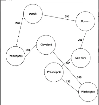
[image:6.612.78.565.196.739.2]

(7)

The suggested tour is Boston-Detroit- Indianapolis-Cleveland-Washington, D.C.-Philadelphia-New York-Boston. The total distance for this tour is 2,052 miles.

Because this is a symmetric TSP- that is, the f r o d t o distance between cities is the same-one could reverse the order of the tour and still have an optimal solution, which covers 2,052 miles.

We show the suggested tour in Figure 2.

zyxwvutsrqponmlkjihgfedcbaZYXWVUTSRQPONMLKJIHGFEDCBA

Other Applications

One can use Excel Solver@ in other applications of the linear programming/zero-one programming approach. For example, suppose that one is aware that major construction projects are underway on the interstate highway sys- tem (in both directions) that connects Boston and New York. Even though the distance between Boston and New York might suggest that certain routes be con- sidered, the construction project might disallow these options. The model can take this into account with the following

two additional constraints:

zyxwvutsrqponmlkjihgfedcbaZYXWVUTSRQPONMLKJIHGFEDCBA

$1$12=O$E$16=0

When these constraints are added, the suggested route is Boston-Philadelphia- New York-Washington, D.C.-Cleve- land-Indianapolis-Detroit-Boston. The distance for this tour is 2,242 miles, or

190 miles longer than the first suggested tour.

Excel Solvero also has a maximiza- tion option. Suppose that one is interest- ed in determining the maximum route through these seven cities. By changing

the MIN option to

zyxwvutsrqponmlkjihgfedcbaZYXWVUTSRQPONMLKJIHGFEDCBA

MAX in the original

spreadsheet from Table 2, one can find the suggested route that gives the long- est tour. That route is Boston-Indian- apolis-New York-Detroit-Philadelphia-

Cleveland-Washington D.C.-Boston, and the distance is 4,020 miles.

Limitations of Solver Model

The standard Solver add-in is limited in the size of model that it can solve. When we attempted to use this algorithm for problems involving more than 10 cities, we observed an error message, indicating that the problem was too large for Solver. Frontline Systems Inc. offers commercial versions of the software that are capable of solving larger problems.

Summary

In this article, we discussed a model designed for solving traveling salesman problems with Microsoft Excel Solvero. Low cost, readily available optimization software can increase the efficiency in formulating and executing linear pro-

gramming problems such as the TSP. Though other useful software add-ins are available, they are more expensive and are not readily available to many operations researchers, business profes- sors, and business practitioners. We used Solver because it is part of the standard Excelo package. There is no additional cost for having Solver; it is already in the software package. The approach that we presented uses a spe-

cial form of the linear programming model, zero-one programming. This approach and the development of spreadsheet templates based on this model should encourage the application of Excel Solver@ and other spreadsheet solutions to a wider range of operations research problems.

REFERENCES

Dantzig, G., Fulkerson, R., &Johnson, S. (1954). Solution of large-scale traveling-salesman

problem.

zyxwvutsrqponmlkjihgfedcbaZYXWVUTSRQPONMLKJIHGFEDCBA

Operations Research. 2, 393-410.

Haag, S.,

zyxwvutsrqponmlkjihgfedcbaZYXWVUTSRQPONMLKJIHGFEDCBA

& Perry, J. (2002). Microsofr Excel

2002 (10.22-10.23).Boston: McGraw-Hill Irwin.

Patterson, M., & Harmel, B. (2002). An algorith- mic approach for solving linear programming transportation problems using Microsoft

Solver. International Journal of Business

zyxwvutsrqponmlkjihgfedcbaZYXWVUTSRQPONMLKJIHGFEDCBA

Disci-

plines, 12(1), 1-5.

Patterson, M., & Harmel, B. (2001). Using Microsoft Excel Solver for linear programming assignment problems. International Journal of

Management, l8(3), 308-3 13.

Robinson, J. B. (1949). On the Hamiltonian Game (a traveling salesman problem). RAND Research Memorandum RM-303.

346 Journal

zyxwvutsrqponmlkjihgfedcbaZYXWVUTSRQPONMLKJIHGFEDCBA

of Education for Business