Childhood
Beck A. Taylor
Eric Dearing
Kathleen McCartney
A B S T R A C T
Prior research has identified statistically significant but small income effects for children’s cognitive, language, and social outcomes. We examine the impact of family economic resources on developmental outcomes in early childhood, the stage of life during which developmental psychologists have suggested income effects should be largest. Using participants from the NICHD Study of Early Child Care, we estimate income effects that are com-parable in absolute terms to those reported in previous research. Relative income effect sizes are found to have practical significance, however, both within our sample, and compared to participation in Early Head Start.
I. Introduction
The association between economic status and children’s cognitive, language, and social development is a contentious issue among those who guide and direct economic and social policies affecting children. If family income has a sub-stantial impact on child development, then transfers of income may play a significant
Beck A. Taylor is an associate professor of economics and the W. H. Smith Professor of Economics at Baylor University. Eric Dearing is an assistant professor of psychology at the University of Wyoming. Kathleen McCartney is a professor of education at the Harvard Graduate School of Education. An earlier version of this paper was presented at the 2001 meetings of the Society for Research in Child Devel-opment. This research was funded in part by a grant from the National Institute of Child Health and Human Development (HD 25451). A portion of Beck Taylor’s work was completed while a visiting scholar at the Harvard Graduate School of Education. The authors would like to thank David Blau, Erdal Tekin, two anonymous referees, and workshop participants at University of Richmond, University of Oregon, and Georgia State University for their valuable comments. The authors would also like to thank Kristen Bub for providing excellent research assistance. The data used in this article can be obtained beginning May 2005 through April 2008 from Beck A. Taylor, Department of Economics, Baylor University, Waco, TX 76798-8003. E-mail: Beck_Taylor@baylor.edu.
[Submitted July 2001; accepted May 2003]
ISSN 022-166XE-ISSN 1548-8004 © 2004 by the Board of Regents of the University of Wisconsin System
role in the development of children living in poverty. On the other hand, if there is little or no effect of family income on child development, then there may be more use-ful strategies for improving the well-being of poor children, for example, direct inter-vention programs such as Head Start.1
Developmental psychologists have written extensively on the links between eco-nomic resources and child outcomes, and most of what has been written concerns issues related to poverty (for reviews see Duncan and Brooks-Gunn 1997, 2000). Economists interested in understanding human capital formation, intergenerational links in economic status, and associated policy implications have recently entered the debate concerning whether poverty negatively impacts child development (see, for example, Blau 1999; Shea 2000; and Aughinbaugh and Gittleman 2001). The discus-sion among economists currently centers on the measurement of economic resources like income, the appropriate set of covariates used to explain variation in child out-comes, methods to control for the potential endogeneity of economic resources, and whether statistical estimates of the association between economic resources and child outcomes have practical importance.
The present study contributes to the existing literature in at least four ways. First, while previous researchers examine outcome measures most often associated with children aged 3–7 years and find that income effects are small, we focus on outcomes measured in early childhood (aged 15–36 months) for which income effects are expected to be larger (Duncan and Brooks-Gunn 1997).
Second, researchers in the past have generally relied upon abbreviated and survey measures of development found in large longitudinal data sets, such as the National Longitudinal Survey of Youth (NLSY) or Panel Study of Income Dynamics (PSID). The data we use, from the National Institute of Child Health and Human Development (NICHD) Study of Early Child Care (SECC), include complete, individually admin-istered performance assessments of cognitive and language development that have superior psychometric properties (in other words, better reliability and validity) than the abbreviated and survey performance instruments found in large longitudinal samples (Sattler 1988; Conoley et al. 1995; Bradley et al. 2001).2
Third, we suggest alternative approaches than those used in previous research for assigning practical importance to estimated income effects. By estimating effect sizes, we present income effects that are large relativeto other predictors, particularly for children who live in poverty. That is, we find that the effect of income is often com-parable to, and sometimes larger than, the effect sizes of other important control vari-ables, such as maternal verbal intelligence. Additionally, we compare our estimated effect sizes to those estimated for early childhood intervention programs, specifically Early Head Start. This comparison suggests that effect sizes associated with changes in family economic resources found herein are similar to those estimated for
partici-1. Note that the effectiveness of direct intervention programs is also debatable. See Currie (1998, 2001) for a review of the literature on early childhood intervention programs.
pation in Early Head Start found elsewhere in the literature (see, for example, U.S. Department of Health and Human Services 2002).
Finally, we examine the potential mediation of the association between family eco-nomic resources and children’s outcomes via the role income likely plays in impact-ing the child’s home environment and maternal depression. In most instances, our results indicate that the home environment and maternal depressive symptoms account for some, but not all, of the variance in child outcomes explained by family income, supporting the notion that there exist other transmission processes through which higher income benefits children.
II. Previous Research
A large empirical literature attempts to estimate the association between family economic status and developmental outcomes.3We focus here on a small, recent set of studies that attempts to control for the potential endogeneity of parental income. Endogeneity of income arises when unobserved heterogeneity across families, parents, and children (and potentially other environmental factors, such as neighborhood characteristics) is correlated with both family income and child outcomes. For example, if unobserved maternal intelligence is correlated with mater-nal income and, through shared genes and a shared home environment, with child out-comes, then the estimated income coefficient will be biased and may not be policy relevant (Blau 1999).4The studies we cite here take important and unique approaches to control for this potential bias.
Using PSID sibling data, Levy and Duncan (2001) estimate the effect of family income on children’s completed years of schooling. They use a family-level (sibling) fixed-effects estimator to control for omitted variables that might be correlated with family income and child outcomes. Although ordinary least squares (OLS) estimates of the effect of income on schooling are small and significantly positive, fixed-effects estimates yield income effects that are even smaller in magnitude and statistically insignificant. Important for our study, when Levy and Duncan extend the analysis to examine the timing of family income during childhood, they find that only family income during early childhood (years 0-4) has a positive and significant effect on schooling.
Ideally, one would test whether family income matters in determining child out-comes by placing money on the doorsteps of randomly selected parents, then track-ing the subsequent development of their children. Ustrack-ing PSID data, Shea (2000) attempts to approximate such an experiment by isolating observable determinants of parents’ income that arguably represent luck (for example, union status,
try, and job loss) and then uses these as instruments for parental income. Although OLS estimates indicate that father’s income plays a significant and positive role in determining future child outcomes such as wages, income, and years of schooling, two-stage least squares estimates reveal that father’s income has no impact on these measures.
Three recent studies are more closely related to our examination in that they exam-ine children’s cognitive, language, and social development rather than future labor market and educational outcomes. In an attempt to distinguish the effect of income from other characteristics, Mayer (1997) utilizes several different measures of in-come (from both the NLSY and PSID), including parental inin-come earned after the outcome was assessed, in models of children’s cognitive and behavioral development. Mayer’s results indicate that future income has a small, positive, and significant effect on child outcomes, with more permanent measures of income (in other words, aver-ages of income over the sample period) having larger effects. As Mayer notes, how-ever, parents’ investment behavior in child outcomes could be forward-looking, making this approach suspect.
Blau (1999) uses the matched mother-child subsample of the NLSY to estimate the impact of income on cognitive and language outcomes for children aged 3–7 years, and motor and social outcomes for children aged 0–3 years. Blau estimates a variety of empirical specifications, including OLS, discrete-factor random effects, and several levels of fixed effects. His findings indicate that OLS estimates of income effects are generally statistically significant and positive, but that the precision of the estimated effects diminishes dramatically when they are estimated using either random- or fixed-effects estimators. Similar to Mayer’s findings, Blau reports that permanent income effects are generally larger in magnitude than contemporaneous income effects. In addition, for most measures examined, Blau does not detect discernable nonlinearities in the income effect—that is, while the marginal impact of an extra dol-lar of income is expected to be greatest at lower levels of income, this result does not emerge from the NLSY data.
Finally, Aughinbaugh and Gittleman (2001) follow Blau’s research design and examine differences in the effect of income on children’s cognitive, language, and social outcomes between children living in the United States and those living in Great Britain. Using the NLSY and Great Britain’s National Child Development Study, Aughinbaugh and Gittleman find that the association between income and children’s developmental outcomes is quite similar for both nations. Discrete-factor random-effects estimates reveal that higher levels of income are associated with better outcomes, but the absolute magnitude of the impact is small.
III. Data and Empirical Methodology
A. DataWe use data from the NICHD Study of Early Child Care (SECC). In 1991, 8,986 women from ten U.S. sites who had recently given birth were visited in hospitals.5Of the 5,151 families who were eligible, 2,352 were invited to participate using a condi-tional random sampling method that ensured that the sample was diverse and repre-sentative of the population with regard to ethnicity, education, and family structure. A total of 1,364 families enrolled in the study, 89 percent (1,216) of whom continued to participate through 36 months.6
The data analyzed here were collected from birth until children were 36 months of age. Demographic information, including child gender, family income data, mother’s education and ethnicity, paternal education, and family structure (the number of adults and children living in the household and mother’s marital status), was collected via mother’s report during home visits when children were one month old.7Data on fam-ily income and famfam-ily structure were then updated during home visits and telephone interviews when children were 6, 15, 24, and 36 months of age. In addition, when children were 36 months old, the mother’s verbal intelligence was assessed using the Peabody Picture Vocabulary Test (PPVT; Dunn and Dunn 1981).8Within the SECC sample, mother’s PPVT demonstrated high reliability as measured by Cronbach’s index of internal consistency (α =0.82). The PPVT has also been validated via cor-relations with the revised Wechsler Adult Intelligence Scale’s (WAIS-R) full scale and subscales (Mangiaracina and Simon 1986).
We measure family economic resources in several ways. Total annual family income, collected at 1, 6, 15, 24, and 36 months, represents income received from all sources, including mother, father/partner (if in the home), and other sources (includ-ing other in-home family members and any government assistance).9Alternatively, a variable measuring family income-to-needs divides total family income by the poverty threshold for the appropriate family size such that a family at the poverty line
5. The ten cities were Little Rock, Ark.; Irvine, Calif.; Lawrence, Kan.; Boston, Mass.; Philadelphia, Penn.; Pittsburgh, Penn.; Charlottesville, Va.; Morganton, N.C.; Seattle, Wash.; and Madison, Wis.
6. There were some demographic differences between families who dropped out of the study and those who continued to participate. Mothers in families who dropped out were less likely to be married and had fewer years of education. Additionally, children in families who withdrew were more likely to be Black (Dearing et al. 2001). Detailed information concerning how the NICHD SECC sample compares with city and U.S. averages is available from the authors upon request.
7. Maternal and paternal education is measured in years of schooling, and maternal ethnicity is measured using dummy variables indicating whether the mother is Black and/or Hispanic.
8. Thus, gender, education, ethnicity, mother’s age at birth, and mother’s PPVT are time invariant in the analyses that follow. Child’s age, number of children and adults living in the home, and mother’s marital status can vary through time.
has an income-to-needs ratio of unity (U.S. Bureau of the Census 1999). Income-to-needs may represent a more accurate picture of the family’s available economic resources as it adjusts income for the living needs of the family.
Both total family income and income-to-needs are measured contemporaneously and as a simple average over the sample period.10Consistent with the previous litera-ture, this averaging of income yields a variable that may represent the family’s “per-manent” income. Because our panel is short (only 36 months) relative to other longitudinal studies that examine distinctions between permanent and contemporane-ous income, our measure of permanent income is likely better interpreted as simply a less noisy measure of income than a true measure of permanent income. We continue to use the term, however, to facilitate comparison across studies.
At 15 and 24 months, children’s cognitive development was measured using the Mental Development Index (MDI) from the Bayley Scales of Infant Development II (Bayley 1993). The MDI has been validated via strong correlations with other meas-ures of children’s intelligence, such as Stanford-Binet IQ (Bayley 1993). The measure is also highly reliable: α =0.80 (Bayley 1993). At 36 months, children’s cog-nitive development was assessed using the School Readiness composite from the Bracken Basic Concept Scale (Bracken 1984). This 51-item measure assesses chil-dren’s abilities in the areas of color recognition, letter identification, number and counting skills, comparisons, and shape recognition. This school readiness composite has demonstrated excellent validity with intelligence measures and academic per-formance in kindergarten (Laughlin 1995; Zucker and Riordan 1988). In the SECC sample, the internal consistency of the measure is excellent (α =0.93).
During laboratory visits at age 36 months, children’s language performance was assessed using the Reynell Developmental Language Scale (Reynell 1991). This 67-item measure is divided into two subscales. The Receptive Language (language comprehension) subscale assesses children’s behavioral responses to verbal requests to identify and manipulate a set of objects—for example, “Put all of the white buttons in the cup.” The Expressive Language subscale assesses children’s speech (for exam-ple, the use of complex sentence structure) and the ability to name and define objects, words, and activities presented pictorially. The Reynell subscales have demonstrated both concurrent and predictive validity via associations with other language measures and intelligence scores (Silva 1986). In the SECC sample, both subscales were inter-nally consistent: α =0.93 for the receptive subscale and α =0.86 for the expressive subscale.
During laboratory visits at 24 and 36 months, children’s social behavior was assessed via maternal report. Specifically, mothers completed both the Child Behavior Checklist (CBCL; Achenbach et al. 1987) and the Adaptive Social Behavior Inven-tory (ASBI; Hogan, Scott, and Bauer 1992). Both of these measures have proven to be valid assessments of children’s behavior via correlations with other behavioral measures and each has demonstrated good internal consistency (Achenbach et al. 1987; Hogan et al. 1992). Based on factor analysis, child behavior composites repre-senting behavior problems (negative behavior) and prosocial behavior (positive
behavior) were formed by summing standardized scores from the subscales of the CBCL and ASBI.11
It should be noted that social scientists have recognized at least two pathways through which income can be transmitted to child outcomes. First, economic resources can be used to invest in opportunities and environments that foster positive outcomes (Blau 1999). Second, economic hardship can translate into parental stress and depression that may in turn adversely affect parent-child interactions (Conger et al. 1997; Elder et al. 1985). To capture environmental effects, the quality of the home environment was assessed at 6, 15, and 36 months using the Home Observation for Measurement of the Environment (HOME; Caldwell and Bradley 1984). Using maternal responses to questions and interviewer observations, this 55-item measure assesses a variety of household characteristics from the quality of parent-child inter-actions to the level of cognitive stimulation available and provided in the home. The HOME measure has been validated via correlations with family social status and maternal IQ (Caldwell and Bradley 1984). Further, the measure has demonstrated excellent reliability (α =0.93). Although the HOME score is not a child outcome measure, estimating the responsiveness of the HOMEscore to changes in income may yield insights into the elasticity of parents’ input demand with respect to changes in income. Thus, we will estimate income effects for not only child outcome measures, but also for the HOMEscore.
Mothers completed the Center for Epidemiological Studies Depression Scale (CES-D; Radloff 1977) at 1, 6, 15, 24, and 36 months. The CES-D is a 20-item check-list measuring the presence and frequency of depressive symptoms in the previous week. Response categories range from zero (rarely or none of the time; in other words, less than once a week) to three (most or all of the time; in other words, 5–7 times a week). One of the most widely used measures of depressive symptoms, the CES-D, has been extensively tested for validity and reliability (Cho et al. 1993). In the SECC sample, reliability ranged from 0.85 to 0.90. The HOMEmeasure described above and maternal depressive symptoms will be used in later analyses that investi-gate the mediating role these variables play in the context of the investment and family stress pathways described above.
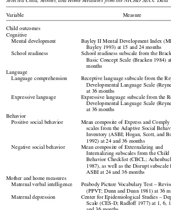
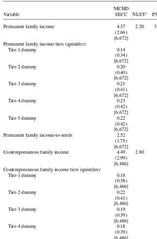
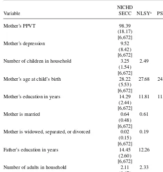
Table 1 summarizes the various measures we use in the analyses to follow. Descriptive statistics for all variables in the SECC sample are reported in Table 2.12 Additionally, we report in Table 2 available sample characteristics from similar stud-ies using the NLSY (Blau 1999) and PSID (Levy and Duncan 2001). Inspection of Table 2 reveals that the SECC sample, as compared to the NLSY and PSID samples,
11. In a principal components factor analysis, the two subscales from the CBCL (Internalizing and Externalizing behavior problems) and three subscales from the ASBI (Comply, Express, and Disrupt) loaded on two factors that cumulatively explained more than 77 percent of the variance in these measures. The load-ings for the first factor, negative behavior, were 0.88 (CBCL: Externalizing), 0.80 (CBCL: Internalizing), and 0.82 (ASBI: Disrupt). The loadings for the second factor, positive behavior, were 0.94 (ASBI: Express) and 0.78 (ASBI: Comply). See NICHD Early Child Care Research Network (1999) for a more detailed description.
is more affluent, contains a smaller proportion of minorities, and has a higher level of parental education, on average. It should be noted that the SECC was not designed to be nationally representative and some low-income groups were deliberately excluded. The liberal use of sample exclusion criteria in the SECC (for example, excluding families from unsafe neighborhoods and mothers not fluent in English) is
Table 1
Selected Child, Mother, and Home Measures from the NICHD SECC Data
Variable Measure
Child outcomes Cognitive
Mental development Bayley II Mental Development Index (MDI; Bayley 1993) at 15 and 24 months School readiness School readiness subscale from the Bracken
Basic Concept Scale (Bracken 1984) at 36 months
Language
Language comprehension Receptive language subscale from the Reynell Developmental Language Scale (Reynell 1991) at 36 months
Expressive language Expressive language subscale from the Reynell Developmental Language Scale (Reynell 1991) at 36 months
Behavior
Positive social behavior Mean composite of Express and Comply sub-scales from the Adaptive Social Behavior Inventory (ASBI; Hogan, Scott, and Bauer 1992) at 24 and 36 months
Negative social behavior Mean composite of Externalizing and Internalizing subscales from the Child Behavior Checklist (CBCL; Achenbach et al. 1987), as well as the Disrupt subscale from the ASBI at 24 and 36 months
Mother and home measures
Maternal verbal intelligence Peabody Picture Vocabulary Test – Revised (PPVT; Dunn and Dunn 1981) at 36 months Maternal depression Center for Epidemiological Studies – Depression
Scale (CES-D; Radloff 1977) at 1, 6, 15, 24, and 36 months
Table 2
Comparative Descriptive Statistics from the NICHD SECC, NLSY, and PSID
NICHD
Variable SECC NLSYa PSIDb
Permanent family income 4.37 2.20 3.19
(2.66) [6,672] Permanent family income tiers (quintiles)
Tier-1 dummy 0.14
(0.34) [6,672]
Tier-2 dummy 0.20
(0.40) [6,672]
Tier-3 dummy 0.21
(0.41) [6,672]
Tier-4 dummy 0.23
(0.42) [6,672]
Tier-5 dummy 0.22
(0.42) [6,672] Permanent family income-to-needs 2.52
(1.75) [6,672] Contemporaneous family income 4.49 2.80
(2.99) [6,486] Contemporaneous family income tiers (quintiles)
Tier-1 dummy 0.18
(0.38) [6,486]
Tier-2 dummy 0.22
(0.41) [6,486]
Tier-3 dummy 0.19
(0.39) [6,486]
Tier-4 dummy 0.18
(0.39) [6,486]
Tier-5 dummy 0.23
Table 2 (continued)
NICHD
Variable SECC NLSYa PSIDb
Contemporaneous family income-to-needs 3.11 (2.34) [6,486]
Poverty dummy (poor) 0.17
(0.38) [6,486] Poverty dummy (ever poor in sample period) 0.32
(0.47) [6,672]
MDI 100.20
(16.49) [2,224]
School readiness 8.95
(2.87) [1,104]
Language comprehension 97.44
(15.75) [1,103]
Expressive language 96.74
(14.58) [1,078]
Negative behavior 0.00
(3.05) [2,187]
Positive behavior 0.00
(1.81) [2,191]
HOME 37.26
(4.67) [3,274]
Child is male 0.52 0.51 0.52
(0.50) [6,672]
Mother is Hispanic 0.04 0.36
(0.20) [6,672]
Mother is Black 0.11 0.22 0.41
Table 2 (continued)
NICHD
Variable SECC NLSYa PSIDb
Mother’s PPVT 98.39
(18.17) [6,672]
Mother’s depression 9.52
(8.42) [6,672] Number of children in household 3.25 2.49
(1.54) [6,672]
Mother’s age at child’s birth 28.22 27.68 24.35 (5.53)
[6,672]
Mother’s education in years 14.29 11.81 11.75 (2.44)
[6,672]
Mother is married 0.64 0.61
(0.48) [6,672] Mother is widowed, separated, or divorced 0.02 0.19
(0.15) [6,672] Father’s education in years 14.45 12.26
(2.60) [6,672] Number of adults in household 2.11 2.33
(0.67) [6,672]
Note: Statistics reported are the mean, (standard deviation), and [sample size]. The SECC descriptive statis-tics are reported for those observations with nonmissing data on mother’s PPVT score. Both permanent and contemporaneous income are measured in 10,000s of 1991 dollars. Income quintiles (tiers) were estimated prior to eliminating observations with missing values for mother’s PPVT score, thus the resulting tiers are not uniformly spaced. Descriptive statistics differ slightly across the usable samples for child outcomes and the HOMEscore. Permanent family income and income-to-needs are averages over all available observations of contemporaneous family income and income-to-needs for a given family. In the regression analysis, child outcomes and the HOMEscore have been divided by their standard deviations.
a. Reported by Blau (1999) and inflated to 1991 dollars.
likely responsible for the disparities noted in Table 2 between the SECC, NLSY, and PSID.
B. Empirical Methodology
Consistent with the previous literature, we estimate reduced-form models that can be written
(1) yijt=Xjtαi+Ijtβi+ ε1ijt,
where yijtis the jth child’s score on the ith assessment in month t, Xis a vector of
regressors, Iis a measure of income, ε1is the disturbance, and αand βare parame-ters to be estimated.13Our six child outcome measures and the HOMEscore, which will serve as our dependent variables, are rescaled by dividing each by its standard deviation (SD) to make regression results across outcomes more easily comparable.
Three of our outcome measures (MDI, negative behavior, and positive behavior) and the HOMEscore have multiple assessments for each child in the SECC data. For the remaining three outcomes (school readiness, language comprehension, and expressive language) we have only one assessment per child. To control for the poten-tial endogeneity of income that is a potenpoten-tial issue for each child outcome and the HOMEscore, regardless of the assessment frequency, we estimate Equation 1 using a discrete-factor model which produces a semi-parametric maximum-likelihood ran-dom-effects estimator identical to that found in Blau (1999) and Aughinbaugh and Gittleman (2001).14,15Although there is sufficient within-family variation in income
13. As stated in Blau (1999), an alternative approach to specifying the reduced-form equation above is to estimate a structural model in which the household maximizes utility by choosing consumption, leisure, and child achievement. A production function that translates inputs of time and other resources into achievement levels could be specified. Estimation of such a model would require strong assumptions given that the SECC data contain no information on family purchases of inputs, such as health care and books, or how outside time is spent.
14. The standard instrumental-variables approach is not feasible in this case because the child outcome equations are reduced form and contain all of the exogenous variables in the model, leaving no instruments to identify the income effect.
15. The discrete factor model requires that income and child outcome equations be estimated jointly, and it will yield consistent estimates of the income effect if income is the only endogenous variable on the right-hand side of the equation. We specify income equations of the form
+
c f2jt,
Ijt=Xjt
and an error structure given by
,
where vand the η’s are independently distributed errors with mean zero, and ρis a factor-loading parame-ter to be estimated. The common factor, v, is defined as the only source of the correlation between Iand ε1 and is integrated out of the model using a full-information maximum-likelihood random-effects estimator. The distribution of the common factor, v, is assumed to be given by the step function
1
to estimate a fixed-effects model, the inability to estimate the impact of permanent family income limits this approach.16
We also estimate Equation 1 using ordinary least squares (OLS), with the standard error estimates associated with our repeated measures of child outcomes adjusted by the Huber-White method to account for nonindependence due to multiple observa-tions per child. Recall that previous researchers have consistently found a reduction in the absolute size (and, in many cases, statistical significance) of estimated income effects when controlling for the potential endogeneity of family income. A compari-son of OLS and random-effects estimates will allow us to identify such changes in the SECC sample if they are present. Regardless of estimation technique, however, we place more faith in estimates of income effects obtained from our repeated measures of child outcomes (MDI, negative behavior, and positive behavior) and the HOME score than in those estimates obtained from our one-time assessments (school readiness, language comprehension, and expressive language).
Because researchers have often disagreed over the appropriate set of covariates to include when estimating the effect of income on child outcomes, for each of our child outcome measures, as well as for the HOMEscore, we estimate three specifications. First, we define a “core” set of regressors that are arguably exogenous. This core set of regressors includes child gender, maternal ethnicity, and child’s age at the time of the assessment. This first specification is guided by the rationale that the policy-relevant, exogenous effect of income is most appropriately estimated when poten-tially endogenous variables that are influenced by, or jointly chosen with, income are excluded from the regression (Blau 1999).
In our second specification, a measure of maternal verbal intelligence (PPVT) is included in addition to predictors from the core set. Including this measure likely con-trols for the influence of mother’s intelligence on income as well as child outcomes. The PPVT score may, however, capture both innate intelligence (ability) as well as endogenous decisions concerning human capital investment (achievement), and, as such, is not included in the core set of regressors exclusively used in the first specification.
In our third specification, in addition to those variables in our second specification, we include a broader set of covariates commonly found in the child development lit-erature (Duncan and Brooks-Gunn 1997). These include the number of children and adults in the household, mother’s age at the child’s birth, maternal and paternal edu-cation, and mother’s marital status. This specification is guided by the rationale that the size of income effects may be overestimated if the variance in child outcomes attributed to income is actually due to conditions, such as education, that are collinear with family economic resources.
the distribution. Because of the lack of identifying instruments, identification is achieved via covariance restrictions, specifically that vis the only source of correlation between Iand ε1, and by setting the factor-loading parameter in ε1equal to unity. For more details, see Heckman and Singer (1984), Mroz and Guilkey (1992), Mroz (1999), Blau (1999), and Aughinbaugh and Gittleman (2001). Other studies to use this approach include Blau and Hagy (1998), Hu (1999), and Mocan and Tekin (2003).
IV. Results
A. Estimated Income EffectsEstimated income effects from Equation 1 are reported in Table 3. For the HOME measure and for each of our six child outcome measures, we report estimated income effects using both permanent income (upper half of Table 3) and contem-poraneous income (lower half). Two measures of income, total family income and income-to-needs, are examined. For each of these measures of income, we report estimates from three separate specifications using the core independent variables, then adding mother’s PPVT score, and finally including other potentially omitted variables commonly used in the child development literature. Both random-effects and OLS [in brackets] estimates are reported.
The first row in Table 3 reveals that in a random-effects model using only our core variables, a $10,000 increase in permanent annual income is associated with an aver-age improvement in child outcomes of 7.3 percent of an SD (recall that lower scores for negative behavior are interpreted as better outcomes), with the largest effect being a nine percent of an SD improvement for school readiness, and the smallest effect being a 5.9 percent of an SD improvement for mental development (MDI). Similarly, a $10,000 increase in permanent annual income is associated with a 10.6 percent of an SD increase in the HOMEscore, larger than any income effect estimated across the six child outcomes. OLS estimates of income effects in the same specification are always larger in absolute magnitude. Specifically, the average income effect across the six outcome measures increases to 9.3 percent of an SD, while the HOME income effect increases to 13.3 percent. That OLS estimates are larger than random-effects estimates is generally consistent throughout the analyses that follow.
The fourth row of Table 3 reports income effects using the same core model, but replaces permanent family income with permanent income-to-needs as our measure of family economic resources. Random-effects estimates reveal that, on average, a one-point increase in the ratio of income to needs leads to a 12.6 percent of an SD improvement across the six child outcome measures, and a 17.8 percent improvement in the HOMEscore. The largest income effect estimated for child outcomes using income-to-needs is 17.3 percent for language comprehension, and the smallest is 9.1 percent for negative behavior. To facilitate a comparison with results generated using permanent family income, we first calculate the average needs in our data to be $17,600 and then multiply each income effect by ($10,000/$17,600). Using the income-to-needs coefficients in this way across the six child outcomes, a $10,000 increase in permanent income translates into an average 7.2 percent of an SD improvement in outcomes and a 10.1 percent of an SD increase in the HOMEscore. Thus, using permanent family income and permanent income-to-needs yields similar estimates of the impact of additional income on developmental outcomes and the home environment.
The Journal of Human Resources
Table 3
Estimated Random-Effects and OLS Coefficients on Linear Income Measuresa
Cognitive Language Behavior
School Language Expressive Negative Positive
Income Measures Model MDIb Readinessc Comprehensionc Languagec Behaviord Behaviord HOMEe
Permanent income measures
Total family income Core 0.059* 0.090* 0.089* 0.069* −0.071* 0.061* 0.106*
[0.085*] [0.109*] [0.116*] [0.090*] [−0.082*] [0.078*] [0.133*]
Total family income Core +mother’s PPVT 0.044* 0.062* 0.053* 0.048* −0.051* 0.037* 0.073*
[0.069*] [0.076*] [0.073*] [0.060*] [−0.071*] [0.060*] [0.094*]
Total family income Core +mother’s PPVT + 0.028* 0.018* 0.021* 0.030* −0.019 0.025* 0.006
others [0.050*] [0.024*] [0.029*] [0.033*] [−0.033*] [0.031*] [0.019]
Income-to-needs Core 0.099* 0.168* 0.173* 0.131* −0.091* 0.096* 0.178*
[0.123*] [0.195*] [0.192*] [0.150*] [−0.111*] [0.125*] [0.213*]
Income-to-needs Core +mother’s PPVT 0.076* 0.111* 0.099* 0.084* −0.057* 0.059* 0.129*
T
aylor
, Dearing, and McCartne
y
995
Total family income Core 0.032* 0.074* 0.075* 0.047* −0.037* 0.033* 0.072*
[0.072*] [0.090*] [0.094*] [0.060*] [−0.059*] [0.056*] [0.110*]
Total family income Core +mother’s PPVT 0.021* 0.049* 0.039* 0.022* −0.026* 0.020* 0.048*
[0.045*] [0.065*] [0.062*] [0.035*] [−0.037*] [0.044*] [0.081*]
Total family income Core +mother’s PPVT + 0.003 0.011 0.018* 0.002 −0.011 0.010 0.005
others [0.028*] [0.023*] [0.030*] [0.006] [−0.019] [0.026*] [0.015]
Income-to-needs Core 0.050* 0.117* 0.112* 0.075* −0.045* 0.047* 0.097*
[0.097*] [0.140*] [0.135*] [0.090*] [−0.066*] [0.071*] [0.127*]
Income-to-needs Core +mother’s PPVT 0.035* 0.084* 0.077* 0.042* −0.029* 0.029* 0.068*
[0.066*] [0.108*] [0.092*] [0.057*] [−0.042*] [0.065*] [0.098*]
Income-to-needs Core +mother’s PPVT + 0.007 0.021* 0.024* 0.001 −0.014 0.015 0.003
others [0.015] [0.039*] [0.045*] [0.003] [−0.023] [0.029*] [0.026]
Note: * indicates statistical significance, p≤0.05. Sample size varies by outcome and specification. a. Both random-effects and OLS [in brackets] coefficients are reported.
b. MDI assessed at 15 and 24 months (average sample size =2,090).
c. School readiness (average sample size =1,055) and language outcomes (average sample size =1,057) assessed at 36 months only. d. Behavioral outcomes assessed at 24 and 36 months (average sample size =2,142).
set of regressors. The corresponding income effect associated with the HOMEscore is 68.9 percent as large. Including the other variables commonly included in the developmental literature results in coefficients that are 49.9 percent as large as those estimated using the core set and mother’s PPVT, and an income effect for the HOME score only 8.2 percent as large (and insignificant). A similar pattern is observed when using income-to-needs. Contrary to several other studies, however, most estimates of the income effect remain statistically significant even after including variables that may be determined simultaneously with income.
Estimates of the effect of changes in contemporaneous income are reported at the bottom of Table 3. As found in previous research, income effects are smaller when current income measures are used. For example, comparing the core model using cur-rent family income to the core model using permanent family income, the average income effect associated with child outcomes decreases by 34.2 percent, and the income effect associated with the HOME score decreases by 32.1 percent. Additionally, for both current total income and current income-to-needs, as one adds more variables to the core model, income effects diminish dramatically and, at times, become insignificant.
Summarizing the results from Table 3, we confirm much of the previous research that estimates income effects associated with child outcomes. Specifically, we report statistically significant effects of income on both child outcomes and the HOME measure, though our estimates are small in absolute size. For instance, using the core model, the estimated (random-effects) income effect for MDI indicates that a $10,000 increase in permanent family income generates a less than one point increase in child IQ. Not surprisingly, including variables that are potentially jointly determined with income reduces the absolute magnitude of the income effect, though our estimates generally remain precise. Income effects associated with permanent income measures are generally greater in magnitude than income effects estimated using contempora-neous income measures. Finally, OLS estimates of income effects are larger than their random-effects counterparts, suggesting that endogeneity is a concern when estimating the association between economic resources and developmental outcomes.
B. Nonlinearities
A common prediction in the child development literature is that economic resources will have smaller marginal impacts on outcomes as these resources increase (Duncan and Brooks-Gunn 1997). Surprisingly, this predicted nonlinearity in the income effect has not been demonstrated robustly in previous findings.17Table 4 presents income effects estimated using two nonlinear specifications. Each model is estimated using the core set of regressors, including mother’s PPVT score, along with the family’s permanent annual income (top portion of Table 4) or the family’s contemporaneous annual income (bottom portion) as the income variable. First, for each outcome
ure and the HOMEscore, we report in Table 4 estimated random-effects and OLS [in brackets] income effects over the poor and nonpoor subsamples through the use of an interaction between a poverty dummy variable and the income measure.18Second, we report income effects estimated across income quintiles in the SECC sample (labeled Tiers 1–5, with Tier 5 being the highest quintile), cutoffs that are arguably less arbitrarily defined than the poverty threshold utilized in the first specification.
Random-effects results reported in Table 4 from the poverty interaction using the permanent measure of income (upper half of Table 4) reveal that changes in income have larger effects within the poor subsample. The average differential impact of a $10,000 increase in permanent income on child outcomes between children living in and out of poverty is 9.1 percent of an SD, with the HOMEscore associated with a 15.3 percent differential. Because a $10,000 increase in income would likely push most in our poor subsample across the poverty threshold, a comparison of propor-tional changes is also warranted. Using the coefficients in Table 4 and means of the poor and nonpoor subsamples to estimate point elasticities, we calculate the percent-age improvement in child outcomes and the HOME score associated with a ten-percent increase in permanent income. For each child outcome and for the HOME score, the estimated income elasticity for the poor subsample exceeds that for the non-poor subsample, and in all but one case (language comprehension) this difference is statistically significant. For example, a ten-percent increase in permanent income for those in poverty yields a 0.12 percent increase in school readiness, but only a 0.07 per-cent increase for those out of poverty. The largest disparity between income elastici-ties occurs for negative behavior. A ten-percent increase in permanent income generates a decline in negative behavior of 1.43 percent and 0.91 percent for the poor and nonpoor groups, respectively. Finally, note that with the exception of negative behavior, we do not detect statistically significant differentials for the poor and non-poor subsamples when using contemporaneous income measures (bottom half of Table 4). The precision of these estimates is likely influenced by the large measure-ment error associated with contemporaneous income relative to the permanent income measure.
With respect to the income-quintile specifications in Table 4, we again see signifi-cant nonlinear effects of permanent (but not contemporaneous) income. The effects of increases in permanent income diminish as one moves up the income ladder, but the point at which diminishing returns begin differs across outcomes. For example, an increase in permanent income does not begin to have a significant differential effect on language comprehension until approximately $61,000 (the 80th percentile), but for both behavioral outcomes, diminishing returns manifest more quickly at approxi-mately $17,000 (the 20th percentile). Point elasticities also suggest diminishing returns to proportional increases in permanent income across the income quintiles.
In summary, both nonlinear specifications reveal that income effects are larger for children living in homes with lower family income, though this relationship is most evident when using a measure of permanent income.
The Journal of Human Resources
Table 4
Estimated Random-Effects and OLS Coefficients on Nonlinear Income Measuresa
Cognitive Language Behavior
Income School Language Expressive Negative Positive
Measures MDIb Readinessc Comprehensionc Languagec Behaviord Behaviord HOMEe
Permanent income measures
Income 0.020 0.081* 0.043* 0.121* 0.041* 0.079* 0.026* 0.096* −0.022 −0.158* 0.011 0.081* 0.021* 0.160*
[0.031] [0.092*] [0.049*] [0.123*] [0.052*] [0.090*] [0.034*] [0.111*] [−0.039] [−0.171*] [0.026] [0.086*] [0.045*] [0.172*]
Income × 0.090* 0.088* 0.049 0.076* −0.165* 0.075* 0.153*
poverty [0.112*] [0.099*] [0.067] [0.086*] [−0.171*] [0.090*] [0.165*]
Income × −0.006 −0.015 0.013 −0.005 0.021* −0.017* −0.046
tier-2 [−0.011] [−0.019] [0.019] [−0.009] [0.029*] [−0.020*] [−0.059]
Income × −0.020 −0.033* −0.009 −0.021* 0.016 −0.021* −0.093*
tier-3 [−0.022] [0.040*] [−0.013] [−0.029*] [0.021*] [−0.026*] [−0.107*]
Income × −0.079* −0.065* −0.024 −0.083* 0.123* −0.071* −0.132*
tier-4 [−0.081*] [−0.069*] [−0.032] [−0.092*] [0.134*] [−0.074*] [−0.133*]
Income × −0.095* −0.105* −0.061* −0.091* 0.186* −0.079* −0.162*
T
aylor
, Dearing, and McCartne
y
999
Income × −0.015 −0.107 −0.056 0.008 −0.153* −0.090 0.016
poverty [0.006] [−0.141] [−0.143] [0.013] [−0.164*] [−0.096] [0.019]
Income × 0.001 −0.010 −0.001 0.005 0.016 0.001 −0.008
tier-2 [0.009] [−0.010] [−0.003] [0.005] [0.018] [0.001] [−0.009]
Income × −0.006 −0.007 0.005 0.003 0.008 0.006 −0.011
tier-3 [−0.006] [−0.009] [0.004] [0.005] [0.010] [0.008] [−0.011]
Income × −0.007 −0.034 −0.010 −0.010 0.088* −0.076 −0.019
tier-4 [−0.008] [−0.038] [−0.012] [−0.011] [0.092*] [−0.081] [−0.021]
Income × −0.019 −0.005 −0.031* −0.009 0.182* −0.101 −0.017
tier-5 [−0.020] [−0.012] [−0.033*] [−0.012] [0.191*] [−0.112] [−0.020]
Note: * indicates statistical significance, p≤0.05. All models are estimated using the core set of regressors, mother’s PPVT score, and main effects of the various categor-ical income or poverty variables. Sample size varies by outcome and specification. Tiers 2–5 represent the top four income quintiles, with Tier-5 being the highest. a. Both random-effects and OLS [in brackets] coefficients are reported.
b. MDI assessed at 15 and 24 months (average sample size =2,090).
c. School readiness (average sample size =1,055) and language outcomes (average sample size =1,057) assessed at 36 months only. d. Behavioral outcomes assessed at 24 and 36 months (average sample size =2,142).
C. Relative Effect Sizes
Studies to date that have examined the association between income and child devel-opmental outcomes have consistently estimated income effects that are small in absolute terms. Our results confirm this finding. When interpreting the magnitude of such estimates, however, it is important to consider that the estimated effects associ-ated with other important predictors of child outcomes are also small in absolute terms. Thus, a potentially useful exercise would be to compare relative effect sizes within the same data set (McCartney and Rosenthal 2000). Unfortunately, economists often give this exercise little attention and dismiss, out of hand, estimates of the income effect on child outcomes as small. When a comparison of relative effects is attempted, previous researchers have not always taken into account the quantitative units in which other predictors of child outcomes are measured. Failing to do so results in the proverbial apples and oranges problem.19Without taking into account the distribution of all predictors, one cannot accurately assess the relative impact of one variable over another.
To estimate more accurately the relative impact of changes in a family’s economic status on children’s development, we repeated the analyses reported in Tables 3 and 4 by regressing child outcomes on z-scores of the predictors in the models. Thus, the resulting standardized coefficients can be interpreted as the effect of a one SD change in the independent variable on our measures of child outcomes. More importantly, estimated coefficients can more easily be compared across regressors in the same model, and relative effects can be correctly determined. Additionally, because among developmental psychologists and statisticians partial correlations are the preferred method of estimating effect size in regression (McCartney and Rosenthal 2000), we also report partial correlations associated with each variable.
Standardized coefficients from a random-effects model and partial correlations [in brackets] using the core set of regressors, including mother’s PPVT and our measure of permanent family income, are reported in Table 5. Given the nonlinearities reported in Table 4, particularly those associated with the poverty threshold, in addition to reporting estimates from the entire sample, we have broken the sample into those chil-dren who live in poverty and those who do not. Additionally, to examine the potential mediating impact of more proximal determinants of development, like the home envi-ronment and maternal depression, we include in Table 5 a second specification that includes these variables on the right-hand side of the estimating equation.20The extent to which income effects are reduced from the first to the second specification will pro-vide some indication of the intervening roles that the home environment (the invest-ment pathway) and maternal depression (the family-stress pathway) play in transmitting the effects of income to children (Baron and Kenny 1986). Significant
income effects still present after accounting for HOME and maternal depression would indicate the existence of additional transmission processes through which higher incomes benefit children, such as neighborhood, school, and childcare quality. Examining first the specifications in Table 5 that do not include the potential inter-vening variables, for the entire sample of children in the SECC data, the effect of permanent family income on child outcomes and the HOMEscore is comparable to other predictors in the estimation. For example, the effect of permanent family income on child outcomes as measured by the standardized coefficients is, on average, 73.5 percent as large as the effect of maternal verbal intelligence (PPVT), a strong predic-tor of child developmental outcomes, and 86 percent as large as maternal PPVT for theHOMEscore.21,22More striking is the relative strength of the income effect for the poor subsample. Again, comparing the effect of permanent income on child outcomes to the effect of mother’s verbal intelligence, the effect size of permanent income is 73.7 percent as large, on average, as maternal PPVT for children living in poor fami-lies, while for the HOMEscore, the effect of income is 30.3 percent largerthan mater-nal PPVT for poor families.23For MDI and negative behavior, the estimated effect size of income is largerthan that of maternal PPVT, though only significantly so for MDI. That is, for one measure of children’s cognitive development, the effect of per-manent family income is greater than that of an accepted determinant (both genetic and environmental) of child outcomes, mother’s verbal intelligence (Ceci et al. 1997; Scarr 1997). For the nonpoor subsample, on the other hand, the income effect is on average 50.1 percent of the effect of mother’s PPVT, while the effect of income is 49.9 percent that of mother’s verbal intelligence for the HOMEscore.24,25
When considering in Table 5 the impact of more proximal determinants of out-comes, like the home environment and maternal depression, we see that in many cases the effect size of permanent income decreases, but remains statistically significant and large relative to maternal verbal intelligence. In addition, the effect of income often compares favorably to either the HOMEscore or maternal depression. When consid-ering the full sample, for example, only income effect sizes for MDI and positive behavior are statistically indistinguishable from zero, and the average income effect size remains 52.7 percent as large as maternal PPVT even after controlling for the home environment and maternal depression. Using the poor and nonpoor subsamples, the average effect size of permanent income is approximately 155 percent larger (driven primarily by the disparity in effect sizes when examining MDI) and 47.2 percent smaller than mother’s verbal intelligence, respectively.
Another method of evaluating the salubrious effects of income is to compare the relative impact of additional income with interventions for children in poverty. The
21. Results are similar using partial correlations.
22. Effect sizes for mother’s PPVT and permanent income estimated from the entire sample are significantly different for MDI, school readiness, language comprehension, positive behavior, and HOME.
23. Using the poor subsample, only negative behavior yields statistically indistinguishable effect sizes for mother’s PPVT and permanent income.
24. From results not reported, we found that permanent income-to-needs is an equally strong predictor of child outcomes and the HOMEscore relative to other control variables (particularly mother’s PPVT) for children living in poverty.
The Journal of Human Resources
Table 5
Comparison of Standardized Coefficients and Relative Effect Sizesa
Cognitive Language Behavior
Income School Language Expressive Negative Positive
Measures MDIb Readinessc Comprehensionc Languagec Behaviord Behaviord HOMEe
All children
Permanent 0.119* 0.013 0.198* 0.137* 0.185* 0.131* 0.150* 0.102* −0.139* −0.058* 0.100* 0.011 0.197*
family [0.130*] [0.012] [0.208*] [0.144*] [0.208*] [0.145*] [0.153*] [0.099*] [−0.125*] [−0.055*] [0.096*] [0.010] [0.206*] income
Mother’s 0.138* 0.062* 0.239* 0.146* 0.315* 0.230* 0.218* 0.147* −0.153* −0.084* 0.190* 0.144* 0.229*
PPVT [0.136*] [0.055*] [0.243*] [0.145*] [0.320*] [0.234*] [0.208*] [0.133*] [−0.131*] [−0.075*] [0.170*] [0.129*] [0.236*]
HOME 0.155* 0.317* 0.289* 0.238* −0.077* 0.152*
[0.136*] [0.311*] [0.299*] [0.219*] [−0.071*] [0.140*]
Mother’s −0.009 −0.017 −0.021 −0.034 0.343* −0.209*
depression [−0.009] [−0.020] [−0.026] [−0.036] [0.340*] [−0.216*]
Poor children
Permanent 0.148* 0.110* 0.179* 0.127* 0.166* 0.111* 0.142* 0.091* −0.199* −0.147* 0.076* 0.006 0.417*
family [0.186*] [0.099*] [0.198*] [0.141*] [0.193*] [0.126*] [0.149*] [0.093*] [−0.197*] [−0.149*] [0.082*] [0.007] [0.279*] income
Mother’s 0.111* 0.017 0.278* 0.186* 0.302* 0.188* 0.250* 0.159* −0.192* −0.153* 0.258* 0.180* 0.320*
PPVT [0.129*] [0.015] [0.287*] [0.184*] [0.308*] [0.187*] [0.244*] [0.143*] [−0.176*] [−0.138*] [0.242*] [0.168*] [0.199*]
HOME 0.205* 0.367* 0.347* 0.279* −0.062 0.202*
[0.183*] [0.362*] [0.347*] [0.259*] [−0.060] [0.198*]
Mother’s −0.060 −0.023 −0.038 −0.062 0.264* −0.204*
T
aylor
, Dearing, and McCartne
y
1003
income
Mother’s 0.123* 0.082* 0.185* 0.129* 0.289* 0.244* 0.166* 0.129* −0.103* −0.057 0.120* 0.120* 0.145*
PPVT [0.125*] [0.079*] [0.202*] [0.132*] [0.315*] [0.260*] [0.172*] [0.124*] [−0.092*] [−0.057] [0.113*] [0.115*] [0.173*]
HOME 0.089* 0.251* 0.239* 0.168* −0.057 0.087*
[0.086*] [0.258*] [0.262*] [0.166*] [−0.059] [0.086*]
Mother’s −0.024 −0.030 −0.003 −0.003 0.377* −0.208*
depression [−0.025] [−0.034] [−0.004] [−0.003] [0.373*] [−0.209*]
Note: * indicates statistical significance, p≤0.05. Sample size varies by outcome and specification. For all specifications that include HOMEand maternal depression, only 36-month outcomes are included, except for MDI which includes only 15-month outcomes. Not included for brevity are standardized coefficients and partial correlations for age of child, child’s gender, and mother’s ethnicity.
a. Both random-effects coefficients and partial correlations [in brackets] are reported. b. MDI assessed at 15 and 24 months (average sample size =1,411).
c. School readiness (average sample size =716) and language outcomes (average sample size =733) assessed at 36 months only. d. Behavioral outcomes assessed at 24 and 36 months (average sample size =1,458).
U.S. Department of Health and Human Services (HHS 2002) reports effect size esti-mates from an experimental evaluation of Early Head Start. This evaluation is a use-ful comparison for our analyses, primarily because children were enrolled from birth through 36 months at which time child outcomes were assessed. HHS examines two outcomes that appear in the SECC data: MDI and negative behavior.26HHS reports that children who participate in Early Head Start experience, on average, a 12.0–14.9 percent of an SD increase in MDI and a 10.2–10.8 percent of an SD decline in nega-tive behavior compared with similar children who did not participate. Our results in Table 5 for poor children, the appropriate comparison group, reveal comparable effects of increases in permanent income. Specifically, a one SD increase in perma-nent income results in a 14.8 percent of an SD improvement in MDI and a 19.9 per-cent of an SD decline in negative behavior. Thus, it appears, at least within the SECC sample, that the effects of redistributional policies designed to permanently increase the financial resources of poor families by approximately $13,108 per year (equiva-lent to a one SD increase in permanent annual income for poor families) would likely be similar to those effects associated with intervention, particularly participation in Early Head Start. Interestingly, the 2002 per-child program cost of Early Head Start, in 1991 dollars, was approximately $13,970 (HHS 2002), only slightly greater than our poor subsample’s standard deviation in permanent annual income.27
In conclusion, although estimates of the impact of family economic resources on child outcomes are small in absolute magnitude, they are large in relative magnitude, both within our study and across studies that examine the effectiveness of interven-tion for children living in poverty. When nonlinearity in, and effect sizes for, the income effect are evaluated, the association between family economic resources and developmental outcomes appears to have practical importance.
V. Conclusion
Economists and developmental psychologists are interested in assess-ing the practical importance of child, family, and neighborhood characteristics in determining children’s cognitive, language, and social development. This paper focuses on the absolute and relative importance of family economic status in the determination of child outcomes and the quality of the home environment for young children. Using a data set from the NICHD Study of Early Child Care that contains state-of-the-art measures of child development, we find that economic resources are important when properly compared with other well-established determinants of devel-opmental outcomes in children, particularly maternal verbal intelligence, and when compared with established interventions, such as Early Head Start. The relative strength of the income effect is even more dramatic for children living in poverty.
26. More specifically, HHS examines only the CBCL as a composite instrument.
With respect to public policy, many have used the small absolute size of estimated income effects to argue that redistributional policy designed to generate enough addi-tional resources to elicit significant improvement in developmental outcomes is pro-hibitive. While this may be the case, mandates concerning the allocation of such additional income that would restrict families in their use of these additional resources (for example, vouchers for high-quality childcare) could yield much larger gains in developmental outcomes than have been measured. Additionally, we argue that researchers should place more emphasis on measuring the relative importance of income, both within and across studies. Although income effects estimated in this study are similar to those estimated by previous researchers, a reasonable accounting of the relative importance of family economic resources, both within our study and compared with Early Head Start, yields far different conclusions.
References
Achenbach, Thomas M., Craig Edelbrock, and Catherine T. Howell. 1987. “Empirically Based Assessment of Behavioral/Emotional Problems of 2- and 3-Year-Old Children.” Journal of Abnormal Child Psychology15(4):629–50.
Aughinbaugh, Alison, and Maury Gittleman. 2001. “Does Money Matter? A Comparison of the Effect of Income on Child Development in the United States and Great Britain.” Unpublished.
Baron, Reuben M., and David A. Kenny. 1986. “The Moderator-Mediator Variable Distinction in Social Psychological Research: Conceptual, Strategic, and Statistical Considerations.” Journal of Personality and Social Psychology51(6):1173–82.
Bayley, Nancy. 1993. Bayley II Scales of Infant Development. New York: Psychological Corporation.
Blau, David M. 1999. “The Effect of Income on Child Development.” Review of Economics and Statistics81(2):261–76.
Blau, David M., and Alison P. Hagy. 1998. “The Demand for Quality in Child Care.” Journal of Political Economy106(1):104–46.
Bracken, Bruce A. 1984. Bracken Basic Concept Scale. San Antonio, Tex.: Psychological Corporation.
Bradley, Robert H., Robert F. Corwyn, Harriette P. McAdoo, and Cynthia Garcia Coll. 2001. “The Home Environments of Children in the United States Part I: Variations by Age, Ethnicity, and Poverty Status.” Child Development72(6):1844–67.
Caldwell, Betty, and Robert Bradley. 1984. Home Observation for Measurement of the Environment. Little Rock, Ark.: University of Arkansas at Little Rock.
Ceci, Stephen J., Tina Rosenblum, Eddy de Bruyn, and Donald Y. Lee. 1997. “A Bio-Ecological Model of Intellectual Development: Moving Beyond H2.” In Intelligence, Heredity, and Environment, ed. R. J. Sternberg and E. Grigorenko, 303–22. New York: Cambridge University Press.
Cho, Maeng J., Eve K. Moscicki, William E. Narrow, and Donald S. Rae. 1993. “Con-cordance between Two Measures of Depression in the Hispanic Health and Nutrition Examination Survey.” Social Psychiatry and Psychiatric Epidemiology28(4):156–63. Conger, Rand D., Katherine J. Conger, and Glen H. Elder. 1997. “Family Economic Hardship
Conoley, Jane C., James C. Impara, and Linda L. Murphy, eds. 1995. The Twelfth Mental Measurements Yearbook. Lincoln, Neb.: Buros Institute of Mental Measurements. Currie, Janet. 1998. “The Effect of Welfare on Child Outcomes.” In Welfare, the Family, and
Reproductive Behavior: Research Perspectives, ed. Robert A. Moffitt, 177–204. Wash-ington, D.C.: National Academy Press.
——— . 2001. “Early Childhood Education Programs.” Journal of Economic Perspectives 15(2):213–38.
Dearing, Eric, Kathleen McCartney, and Beck A. Taylor. 2001. “Change in Family Income-to-Needs Matters More for Children With Less.” Child Development72(6):1779–93. Duncan, Greg J., and Jeanne Brooks-Gunn. 1997. “Income Effects across the Life Span:
Integration and Interpretation.” In Consequences of Growing Up Poor, ed. Greg J. Duncan and Jeanne Brooks-Gunn, 596–610. New York: Russell Sage Foundation.
———. 2000. “Family Poverty, Welfare Reform, and Child Development.” Child Devel-opment71(1):188–96.
Dunn, L.M., and L.M. Dunn. 1981. Peabody Picture Test—Revised Manual for Forms L and M. Circle Pines, Minn.: American Guidance Service.
Elder, Glen H., Tri V. Nguyen, and Avshalom Caspi. 1985. “Linking Economic Hardship to Children’s Lives.” Child Development56(2):361–75.
Heckman, James J., and Burton Singer. 1984. “A Method for Minimizing the Impact of Distributional Assumptions in Economic Models for Duration Data.” Econometrica 52(2):271–320.
Hogan, Anne E., Keith G. Scott, and Charles R. Bauer. 1992. “The Adaptive Social
Behavior Inventory (ASBI): A New Assessment of Social Competence in High-Risk Three-Year-Olds.” Journal of Psychoeducational Assessment10(3):230–39.
Hu, Wei-Yin. 1999. “Child Support, Welfare Dependency, and Women’s Labor Supply.” Journal of Human Resources34(1):71–103.
Laughlin, Timothy. 1995. “The School Readiness Composite of the Bracken Basic Concept Scale as an Intellectual Screening Instrument.” Journal of Psychoeducational Assessment 13(3):294–302.
Levy, Dan, and Greg J. Duncan. 2001. “Using Sibling Samples to Assess the Effect of Childhood Family Income on Completed Schooling.” Unpublished.
Mangiaracina, John, and Michael J. Simon. 1986. “Comparison of the PPVT-R and WAIS-R in State Hospital Psychiatric Patients.” Journal of Clinical Psychology42(5):817–20. Mayer, Susan. 1997. What Money Can’t Buy: Family Income and Children’s Life Chances.
Cambridge, Mass.: Harvard University Press.
McCartney, Kathleen, and Robert Rosenthal. 2000. “Effect Size, Practical Importance, and Social Policy for Children.” Child Development71(1):173–80.
Mocan, H. Naci, and Erdal Tekin. 2003. “Nonprofit Sector and Part-Time Work: An Analysis of Employer-Employee Matched Data of Child Care Workers.” Review of Economics and Statistics, Forthcoming.
Mroz, Thomas A. 1999. “Discrete Factor Approximation in Simultaneous Equation Models: Estimating the Impact of a Dummy Endogenous Variable on a Continuous Outcome.” Journal of Econometrics92(2):193–232.
Mroz, Thomas A., and David Guilkey. 1992. “Discrete Factor Approximations for Use in Simultaneous Equation Models with both Continuous and Discrete Endogenous Variables.” Published.
NICHD Early Child Care Research Network. 1999. “Child Outcomes When Child Care Center Classes Meet Recommended Standards for Quality.” American Journal of Public Health89(7):1072–77.
Reynell, Joan. 1991. Reynell Developmental Language Scales(U.S. ed.). Los Angeles: Western Psychological Service.
Sattler, Jerome M. 1988. Assessment of Children(3 ed.). San Diego, CA: Sattler.
Scarr, Sandra. 1997. “Behavior-Genetic and Socialization Theories of Intelligence: Truce and Reconciliation.” In Intelligence, Heredity, and Environment, ed. R. J. Sternberg and E. Grigorenko, 3–41. New York: Cambridge University Press.
Shea, John. 2000. “Does Parents’ Money Matter?” Journal of Public Economics 77(2):155–84.
Silva, Phil A. 1986. “A Comparison of the Predictive Validity of the Reynell Development Language Scales, the Peabody Picture Vocabulary Test and the Stanford-Binet Intelligence Scale.” British Journal of Educational Psychology56(2):201–04.
U.S. Bureau of the Census. 1999. Poverty Thresholds. Washington, D.C.: U.S. Census. U.S. Department of Health and Human Services. 2002. Making a Difference in the Lives of
Infants and Toddlers and Their Families: The Impacts of Early Head Start: Executive Summary. Washington, D.C.: HHS.
Weinberg, Bruce A. 2001. “An Incentive Model of the Effect of Parental Income on Children.” Journal of Political Economy109(2):266–80.