Interactive Segmentation Techniques Free ebook download

(1)

S P R I N G E R B R I E F S I N E L E C T R I C A L A N D

C O M P U T E R E N G I N E E R I N G 

S I G N AL P R O C ES S IN G

Jia He

Chang-Su Kim

C.-C. Jay Kuo

Interactive

Segmentation

Techniques

Algorithms and

Performance

(2)

SpringerBriefs in Electrical and Computer

Engineering

Signal Processing

Series Editor

C.-C. Jay Kuo, Los Angeles, USA Woon-Seng Gan, Singapore, Singapore

For further volumes:

(3)

Jia He

•

Chang-Su Kim

•

C.-C. Jay Kuo

Interactive Segmentation

Techniques

Algorithms and Performance Evaluation

(4)

Jia He

Department of Electrical Engineering University of Southern California Los Angeles, CA

USA

Chang-Su Kim

School of Electrical Engineering Korea University

Seoul

Republic of South Korea

C.-C. Jay Kuo

Department of Electrical Engineering University of Southern California Los Angeles, CA

USA

ISSN 2196-4076 ISSN 2196-4084 (electronic) ISBN 978-981-4451-59-8 ISBN 978-981-4451-60-4 (eBook) DOI 10.1007/978-981-4451-60-4

Springer Singapore Heidelberg New York Dordrecht London

Library of Congress Control Number: 2013945797

Ó_{The Author(s) 2014}

This work is subject to copyright. All rights are reserved by the Publisher, whether the whole or part of the material is concerned, specifically the rights of translation, reprinting, reuse of illustrations, recitation, broadcasting, reproduction on microfilms or in any other physical way, and transmission or information storage and retrieval, electronic adaptation, computer software, or by similar or dissimilar methodology now known or hereafter developed. Exempted from this legal reservation are brief excerpts in connection with reviews or scholarly analysis or material supplied specifically for the purpose of being entered and executed on a computer system, for exclusive use by the purchaser of the work. Duplication of this publication or parts thereof is permitted only under the provisions of the Copyright Law of the Publisher’s location, in its current version, and permission for use must always be obtained from Springer. Permissions for use may be obtained through RightsLink at the Copyright Clearance Center. Violations are liable to prosecution under the respective Copyright Law. The use of general descriptive names, registered names, trademarks, service marks, etc. in this publication does not imply, even in the absence of a specific statement, that such names are exempt from the relevant protective laws and regulations and therefore free for general use.

While the advice and information in this book are believed to be true and accurate at the date of publication, neither the authors nor the editors nor the publisher can accept any legal responsibility for any errors or omissions that may be made. The publisher makes no warranty, express or implied, with respect to the material contained herein.

Printed on acid-free paper

(5)

Dedicated to my parents and my husband,

for their love and endless support

—Jia

Dedicated to Hyun, Molly, and Joyce

—Chang-Su

Dedicated to my wife for her long-term

understanding and support

(6)

Preface

Image segmentation is a key technique in image processing and computer vision, which extracts meaningful objects from an image. It is an essential step before people or computers perform any further processing, such as enhancement, editing, recognition, retrieval and understanding, and its results affect the performance of these applications significantly. According to the requirement of human interac-tions, image segmentation can be classified into interactive segmentation and automatic segmentation. In this book, we focus on Interactive Segmentation Techniques, which have been extensively studied in recent decades. Interactive segmentation emphasizes clear extraction of objects of interest, whose locations are roughly indicated by human interactions based on high level perception. This book will first introduce classic graph-cut segmentation algorithms and then dis-cuss state-of-the-art techniques, including graph matching methods, region merging and label propagation, clustering methods, and segmentation methods based on edge detection. A comparative analysis of these methods will be pro-vided, which will be illustrated using natural but challenging images. Also, extensive performance comparisons will be made. Pros and cons of these inter-active segmentation methods will be pointed out, and their applications will be discussed.

(7)

Chapter 1

Introduction

Keywords Interactive image segmentation

·

Automatic image segmentation

·

Object extraction

·

Boundary tracking

Image segmentation, which extracts meaningful partitions from an image, is a criti-cal technique in image processing and computer vision. It finds many applications, including arbitrary object extraction and object boundary tracking, which are basic image processing steps in image editing. Furthermore, there are application-specific image segmentation tasks, such as medical image segmentation, industrial image segmentation for object detection and tracking, and image and video segmentation for surveillance [1–5]. Image segmentation is an essential step in sophisticated visual processing systems, including enhancement, editing, composition, object recognition and tracking, image retrieval, photograph analysis, system controlling and vision un-derstanding. Its results affect the overall performance of these systems significantly [2,6–8].

To comply with a wide range of application requirements, a substantial amount of research on image segmentation has been conducted to model the segmentation problem, and a large number of methods have been proposed to implement segmen-tation systems for practical usage. The task of image segmensegmen-tation is also referred to as object extraction and object contour detection. Its target can be one or multi-ple particular objects. The characteristics of target objects, such as brightness, color, location, and size, are considered as “objectiveness”, which can be obtained automat-ically based on statistical prior knowledge in an unsupervised segmentation system or be specified by user interaction in an interactive segmentation system. Based on different settings of objectiveness, image segmentation can be classified into two main types: automatic and interactive [9].

(10)

2 1 Introduction

In most cases, it is difficult for a computer to determine the “objectiveness” of the segmentation. In the worst case, even with clearly specified “objectiveness,” the contrast and luminance of an image is very low and the desired object has similar colors with background, which may produce weak and ambiguous edges along object boundaries. Under these situations, automatic segmentation may fail to capture user intention and produce meaningful segmentation results.

To impose constraints on the segmentation, interactive segmentation involves user interaction to indicate the “objectiveness” and thus to guide an accurate seg-mentation. This can generate effective solutions even for challenging segmentation problems. With prior knowledge of objects (such as brightness, color, location, and size) and constraints indicated by user interaction, segmentation algorithms often generate satisfactory results. A variety of statistical techniques has been introduced to identify and describe segments to minimize the bias between different segmen-tation results. Most interactive segmensegmen-tation systems provide an iterative procedure to allow users to add control on temporary results until a satisfactory segmentation result is obtained. This application requires the system to process quickly and update the result immediately for further refinement, which in turn demands an acceptable computational complexity of interactive segmentation algorithms.

A classic image model is to treat an image as a graph. One can build a graph based on the relations between pixels, along with prior knowledge of objects. The most commonly used graph model in image segmentation is the Markov random field (MRF), where image segmentation is formulated as an optimization problem that optimizes random variables, which correspond to segmentation labels, indexed by nodes in an image graph. With prior knowledge of objects, the maximum a posteriori (MAP) estimation method offers an efficient solution. Given an input image, this is equivalent to minimizing an energy cost function defined by the segmentation posterior, which can be solved by graph-cut [10, 11], the shortest path [12, 13], random walks [14,15], etc. Another research activity has targeted at region merging and splitting with emphasis on the completion of object regions. This approach relies on the observation that each object is composed of homogeneous regions while background contains distinct regions from objects. The merging and splitting of regions can be determined by the statistical hypothesis techniques [16–18].

The goal of interactive segmentation is to obtain accurate segmentation results based on user input and control while minimizing interaction effort and time as much as possible [19,20]. To meet this goal, researchers have proposed various solutions and their improvements [18, 21–24]. Their research has focused on algorithmic efficiency and satisfactory user interaction experience. Some algorithms have been developed as practical segmentation tools. Examples include the Magnetic Lasso Tool, the Magic Wand Tool, and the Quick Select Tool in the Adobe Photoshop [25], and the Intelligent Scissors [26] and the Foreground Select Tool [27,28] in another imaging program GIMP [29].

(11)

1 Introduction 3

weaknesses of several representative methods in practical applications so as to pro-vide a guidance to users. Users should be able to select proper methods for their applications and offer simple yet sufficient input signals to the segmentation system to achieve the segmentation task. Furthermore, discussion on drawbacks of these methods may offer possible ways to improve these techniques.

We are aware of several existing survey papers on interactive image segmentation techniques [6,7,32,33]. However, they do not cover the state-of-the-art techniques developed in the last decade. We describe both classic segmentation methods as well as recently developed methods in this book. This book provides a comprehensive updated survey on this fast growing topic and offers thorough performance analysis. Therefore, it can equip readers with modern interactive segmentation techniques quickly and thoroughly.

The remainder of this book is organized as follows. In Chap.2, we give an overview of interactive image segmentation systems, and classify them into several types. In Chap.3, we begin with the classic graph-cut algorithms and then introduce several state-of-the-art techniques, including graph matching, region merging and label prop-agation, clustering methods, and segmentation based on edge detection. In Chap.4, we conduct a comparative study on various methods with performance evaluation. Some test examples are selected from natural images in the database [34] and Flickr images (http://www.flickr.com). Pros and cons of different interactive segmentation methods are pointed out, and their applications are discussed. Finally, concluding remarks on interactive image segmentation techniques and future research topics are given in Chap.5.

References

1. Bai X, Sapiro G (2007) A geodesic framework for fast interactive image and video segmentation and matting. In: IEEE 11th international conference on computer vision, ICCV 2007, IEEE, pp. 1–8

2. Grady L, Sun Y, Williams J (2006) Three interactive graph-based segmentation methods applied to cardiovascular imaging. In: Paragios N, Chen Y, Faugeras O (eds) Handbook of Mathematical Models in Computer Vision. Springer, pp. 453–469

3. Ruwwe C, Zölzer U (2006) Graycut-object segmentation in ir-images. In: Bebis G, Boyle R, Parvin B, Koracin D, Remagnino P, Nefian AV, Gopi M, Pascucci V, Zara J, Molineros J, Theisel H, Malzbender T (eds) Proceedings of Second International Symposium on Advances in Visual Computing, ISVC 2006, Nov 6–8, vol 4291. Springer, pp 702–711, ISBN: 3-540-48628-3,http://researchr.org/publication/RuwweZ06, doi:10.1007/11919476_70

4. Steger S, Sakas G (2012) Fist: fast interactive segmentation of tumors. Abdominal Imaging. Comput Clin Appl 7029:125–132

5. Sommer C, Straehle C, Koethe U, Hamprecht FA (2011) ilastik: interactive learning and seg-mentation toolkit. In: 8th IEEE international symposium on biomedical imaging (ISBI 2011) 6. Ikonomakis N, Plataniotis K, Venetsanopoulos A (2000) Color image segmentation for

multi-media applications. J Intel Robot Syst 28(1):5–20

7. Luccheseyz L, Mitray S (2001) Color image segmentation: A state-of-the-art survey. Proc Indian Natl Sci Acad (INSA-A) 67(2):207–221

(12)

4 1 Introduction

9. McGuinness K, O’Connor N (2010) A comparative evaluation of interactive segmentation algorithms. Pattern Recogn 43(2):434–444

10. Boykov Y, Jolly M (2001) Interactive graph cuts for optimal boundary and region segmentation of objects in nd images. In: Eighth IEEE international conference on computer vision, 2001. ICCV 2001, IEEE, vol 1, pp. 105–112

11. Boykov Y, Veksler O (2006) Graph cuts in vision and graphics: theories and applications. In: Handbook of Mathematical Models in Computer Vision pp 79–96

12. Mortensen E, Barrett W (1998) Interactive segmentation with intelligent scissors. Graph Models Image Proces 60(5):349–384

13. Mortensen E, Morse B, Barrett W, Udupa J (1992) Adaptive boundary detection using ‘live-wire’ two-dimensional dynamic programming. In: Computers in Cardiology 1992. Proceed-ings, IEEE, pp. 635–638

14. Grady L (2006) Random walks for image segmentation. IEEE Trans Pattern Anal Mach Intel 28(11):1768–1783

15. Kim T, Lee K, Lee S (2008) Generative image segmentation using random walks with restart. Comput Vision-ECCV 2008:264–275

16. Adams R, Bischof L (1994) Seeded region growing. IEEE Trans Pattern Anal Mach Intel 16(6):641–647

17. Mehnert A, Jackway P (1997) An improved seeded region growing algorithm. Pattern Recogn Lett 18(10):1065–1071

18. Ning J, Zhang L, Zhang D, Wu C (2010) Interactive image segmentation by maximal similarity based region merging. Pattern Recogn 43(2):445–456

19. Malmberg F (2011) Graph-based methods for interactive image segmentation. Ph.D. thesis, University West

20. Shi R, Liu Z, Xue Y, Zhang X (2011) Interactive object segmentation using iterative adjustable graph cut. In: Visual communications and image processing (VCIP), IEEE, 2011, pp 1–4 21. Calderero F, Marques F (2010) Region merging techniques using information theory statistical

measures. IEEE Trans Image Proces 19(6):1567–1586

22. Couprie C, Grady L, Najman L, Talbot H (2009) Power watersheds: a new image segmentation framework extending graph cuts, random walker and optimal spanning forest. In: 2009 IEEE 12th international conference on computer vision, pp 731–738. IEEE

23. Falcão A, Udupa J, Miyazawa F (2000) An ultra-fast user-steered image segmentation para-digm: live wire on the fly. IEEE Trans Med Imag 19(1):55–62

24. Noma A, Graciano A, Consularo L, Bloch I (2012) Interactive image segmentation by matching attributed relational graphs. Pattern Recogn 45(3):1159–1179

25. Collins LM (2006) Byu scientists create tool for “virtual surgery”. Deseret Morning News pp 07–31

26. Mortensen EN, Barrett WA (1995) Intelligent scissors for image composition. In: Proceedings of the 22nd annual conference on Computer graphics and interactive techniques, SIGGRAPH ’95, pp. 191–198. ACM, New York (1995)

27. Friedland G, Jantz K, Rojas R (2005) Siox: simple interactive object extraction in still images. In: Seventh IEEE international symposium on multimedia, p 7. IEEE

28. Friedland G, Lenz T, Jantz K, Rojas R (2006) Extending the siox algorithm: alternative cluster-ing methods, sub-pixel accurate object extraction from still images, and generic video segmen-tation. Free University of Berlin, Department of Computer Science, Technical report B-06-06 29. Gimp G (2008) Image manipulation program. User manual, Edge-detect filters, Sobel, The

GIMP Documentation Team

30. Lombaert H, Sun Y, Grady L, Xu C (2005) A multilevel banded graph cuts method for fast image segmentation. In: Tenth IEEE international conference on computer vision, 2005. ICCV, vol 1, pp 259–265. IEEE

31. McGuinness K, OConnor NE (2011) Toward automated evaluation of interactive segmentation. Comput Vis Image Underst 115(6):868–884

(13)

References 5

33. Gauch J, Hsia C (1992) Comparison of three-color image segmentation algorithms in four color spaces. In: Applications in optical science and engineering, pp 1168–1181. International Society for Optics and Photonics

(14)

Chapter 2

Interactive Segmentation: Overview

and Classification

Keywords Graph modeling

·

Markov random field

·

Maximum a posteriori

·

Boundary tracking

·

Label propagation

Being different from automatic image segmentation, interactive segmentation allows user interaction in the segmentation process by providing an initialization and/or feedback control. A user-friendly segmentation system is required in practical appli-cations. Many recent developments have driven interactive segmentation techniques to be more and more efficient. We give an overview on the design of interactive segmentation systems, commonly-used graphic models and classification of seg-mentation techniques in this chapter.

2.1 System Design

A functional view of an interactive image segmentation system is depicted in Fig.2.1. It consists of the following three modules:

• User Input Module (Step 1)

This module receives user input and/or control signals, which helps the system recognize user intention.

• Computational Module (Step 2)

This is the main part of the system. The segmentation algorithm runs automatically according to user input and generates intermediate segmentation results.

• Output Display Module (Step 3)

The module delineates and displays the intermediate segmentation results.

The above three steps operate in a loop [1]. In other words, the system allows addi-tional user feedback after Step 3, and then it is back to Step 1. The system runs iteratively until the user gets a satisfied result and terminates the process.

J. He et al.,Interactive Segmentation Techniques, 7 SpringerBriefs in Signal Processing

(15)

8 2 Interactive Segmentation: Overview and Classification

Fig. 2.1 Illustration of an interactive image segmentation system [1], where a user can control the process iteratively until a satisfactory result is obtained

Fig. 2.2 The process of an interactive segmentation system

The process of an interactive image segmentation system is shown in Fig. 2.2, where the segmentation objectives rely on human intelligence. Such knowledge is offered to the system via human interaction, which is represented in the form of draw-ing that provides the color, texture, location, and size information. The interactive segmentation system attempts to understand user intention based on the high-level information so that it can extract the accurate object regions and boundaries even-tually. In the process, the system may update and improve the segmentation results through a series of interactions. Thus, it is a human–machine collaborative method-ology. On one hand, a machine has to interpret user input and segments the image through an algorithmic process. On the other hand, a user should know how his/her input will affect machine behavior to save the iterations.

(16)

2.1 System Design 9

According to Grady [3], an ideal interactive segmentation system should satisfy the following four properties:

• Fast computation in the computational module;

• Fast and easy editing in the user input module;

• Ability to generate an arbitrary segmentation contour given sufficient user control;

• Ability to provide intuitive segmentation results.

Research on interactive segmentation system design has focused on enhancing these four properties. Fast computation and user-friendly interface modules are essen-tial requirements for a practical interactive segmentation system, since an user should be able to sequentially add or remove strokes/marks based on updated segmentation results in real time. This implies that the computational complexity of an interactive image segmentation algorithm should be at an acceptable level. Furthermore, the system should be capable of generating desired object boundaries accurately with a minimum amount of user effort.

2.2 Graph Modeling and Optimal Label Estimation

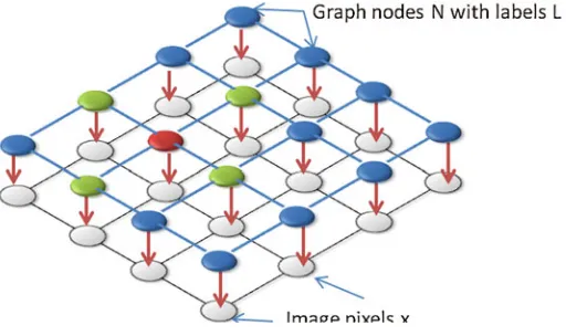
Image segmentation aims to segment out user’s desired objects. Target may consist of multiple homogeneous regions whose pixels share some common properties while the discontinuity of brightness, colors, contrast and texture of image pixels indicates the location of object boundaries [4]. Segmentation algorithms have been developed using the features of pixels, the relationship between pixels and their neighbors, etc. To study these features and connections, one typical approach is to model an input image as a graph, where each pixel corresponds to a node [5].

A graph, denoted byG=(V,E), is a data structure consisting of a set of nodes

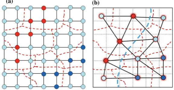
Vand a set of edgesEconnecting those nodes [5]. If an edge, which is also referred to as a link, has a direction, the graph is called a directed graph. Otherwise, it is an undirected graph. We often model an image as an undirected graph and use a node to represent a pixel in the image. Since each pixel in an image is connected with its neighbors, such as 4-connected neighborhood or 8-connected neighborhood as shown in Fig. 2.3, its associated graph model is structured in the same way. An edge between two nodes represents the connection of these two nodes. In some cases, we may treat an over-segmented region as a basic unit, called the superpixel [6–9], and use a node to represent the superpixel.

An implicit assumption behind the graph approach is that, for a given image

I, there exists a probability distribution that can capture labels of nodes and their relationship [10]. Specifically, let node x in graph G be associated with random variablelfrom setL, which indicates its segmentation status (foreground object or background), the problem of segmenting imageIis equivalent to a labeling problem of graphG.

(17)

Fig. 2.3 A simple graph example of a 4×4 image. Therednode has 4greenneighbors in (a) and 8greenneighbors in (b).aGraph with 4-connected neighborhood.bGraph with 8-connected neighborhood

• Pairwise Markov independence.

• Any two non-adjacent variables are conditionally independent given all other vari-ables. Mathematically, for non-adjacent nodesxi andxj (i.e.ei,j ∈ E), labelli

andlj are independent when conditioned on all other variables:

Pr(li,lj|LV\{i,j})=Pr(li|LV\{i,j})Pr(lj|LV\{i,j}). (2.1)

• Local Markov independence.

Given the neighborhoodN _{of node} xi, its labelli is independent of the rest of

other labels:

Pr(li|LV\{i})= Pr(li|LN(i)). (2.2)

• Global Markov property.

• SubsetsAandBof Lare conditionally independent given a separating subsetS, where every path connecting a node inAand a node inBpasses throughS.

If the above properties hold, the graph of image I can be modeled as a Markov random field (MRF) under the Bayesian framework. Figure 2.4shows the MRF of a 4×4 image with 4-connected neighborhood.

Since image segmentation can be formulated as a labeling problem in an MRF, the task becomes the determination of optimal labels for nodes in the MRF. Some node labels are set through user interactions in interactive image segmentation. With the input image as well as this prior knowledge, the maximum a posteriori (MAP) method provides an effective solution to the label estimation of the remaining nodes in the graph [5,10,11]. According to the Bayesian rule, the posterior probability of node labels can be written as

Pr(l1···N|x1···N)=

N

i=1Pr(xi|li)Pr(l1···N)

Pr(x1···N)

(18)

2.2 Graph Modeling and Optimal Label Estimation 11

Fig. 2.4 The MRF model of a 4×4 image

where Pr(l)is the prior probability of labels andPr(x|l)is the conditional proba-bility of the node value conditioned on a certain label.

In the MAP estimation, we search for labelslˆ1···N that maximize the posterior

probability:

ˆ

l1···N =arg max l1···N

Pr(l1···N|x1···N)

=arg max

l1···N

N

i=1

Pr(xi|li)Pr(l1···N)

=arg max

l1···N

N

i=1

log[Pr(xi|li)] +log[Pr(l1···N)] (2.4)

By using the pairwise Markov property and the clique potential of the MRF, we have

Pr(l1···N)∝exp(−

(i,j)∈E

E2(i,j)), (2.5)

whereE2is the pairwise clique potential. It can be regarded as an energy function to measure the compatibility of neighboring labels [5]. In the segmentation literature, it is also called the smoothness term or the boundary term because of its physical meaning in the segmentation [1,12,13].

The first term in Eq. (2.4) is a log likelihood function. By following Eq. (2.4) and with the following association

(19)

which is referred to as the data term or the regional term [1,12,13], we can define the total energy function as

E(l1···N)=

i∈V

E1(i)+

(i,j)∈E

E2(i,j). (2.7)

Then, the MAP estimation problem is equivalent to the minimization of the energy functionE:

ˆ

l1···N =arg min l1···N

i∈V

E1(i)+

(i,j)∈E

E2(i,j). (2.8)

The set L of labels that minimizes energy function E yields the optimal solution. Finally, segmentation results can be obtained by extracting pixels or regions associ-ated with the foreground labels. We will present several methods to solve the above energy minimization problem in Chap.3.

2.3 Classification of Solution Techniques

One can classify interactive segmentation techniques into several types based on different viewpoints. They are discussed in detail below.

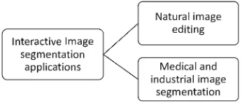
• Application-Driven Segmentation

One way to classify interactive segmentation methods is based on their applica-tions. Some techniques target at generic natural image segmentation, while others address medical and industrial image applications as shown in Fig. 2.5. Natural images tend to have rich color information, which offer a wide range of inten-sity features for the segmentation purpose. The challenges lie in weak boundaries and ambiguous objects. An ideal segmentation method should be robust in han-dling a wide variety of images consisting of various color intensity, luminance, object size, object location, etc. Furthermore, no shape prior is used. In contrast, for image segmentation in medical and industrial applications, most images are monochrome and segmentation objects are often specific such as cardiac cells [14], neuron [15], and brain and born CT [3]. Without the color information, medical image segmentation primarily relies on the luminance information. It is popular

(20)

2.3 Classification of Solution Techniques 13

to learn specific object shape priors to add more constraints so as to cut out the desired object.

• Mathematical Models and Tools

Another way to classify image segmentation methods is based on the mathematical models and tools. Graph models were presented in Sect.2.2. Other models and tools include Bayesian theory, Gaussian mixture models [6], Gaussian mixture Markov random fields [16], Markov random fields [10], random walks [3], random walks with restart [17], min-cut/max-flow [12,18], cellular automation [19], belief propagation [20], and spline representation [21].

• Form of Energy Function

Another viewpoint is to consider the form of the energy function. Generally, the energy function consists a data term and a smoothness term. The data term rep-resents labeled image pixels or superpixels of objects and background defined through user interactions. The smoothness term specifies local relations between pixels or super pixels with their neighborhood (such as color similarity and the edge information). The combined energy function should strike a balance between those two terms. The mathematical tool for energy minimization and the similarity measure also provides a categorization tool for segmentation methods.

• Local Versus Global Optimization

It is typical to adopt one of the following two approaches to minimize the energy function. One is to find the local discontinuity of the image amplitude attribut-ion to locate the boundary of a desired object and cut it out directly. The other is to model the image as a probabilistic graph and use some prior information (such as user scribbles, shape priors, or even learned models) to determine the labels of remaining pixels under some global constraints. Commonly used oper-ations include classification, clustering, splitting and merging, and optimization. The global constraints are used to generate smooth and desired object regions by connecting neighboring pixels of similar attributes and separating pixels in dis-continuous regions (i.e., boundary regions between objects and the background) as much as possible. Here, a graph model is built to capture not only the color features of pixels but also the spatial relationship between adjacent pixels. The global optimization should consider these two kinds of relations. Image segmen-tation approaches also vary on the definitions of the attributions of the probabilis-tic graphs and the measurements of feature similarities between local connected nodes.

• Pixel-wise Versus Region-wise Processing

(21)

Fig. 2.6 A graph model for a 7×7 image with over-segmentation. Homogeneous pixels are merged into a superpixel, and then represented as a node in the graph in (b), where edges connect neighboring superpixels in (a).aImage with oversegmentation.bGraph based on superpixels

the processing time of large images significantly. On the other hand, it may cause errors near object boundaries. Since the segmentation is based on superpixels, it is challenging to locate accurate boundaries. For objects with soft boundaries, a hard boundary segmentation is not acceptable. Then, a post-segmentation procedure is needed to refine object boundaries. Image matting [6,8,20,22] can be viewed as a post-processing technique as well.

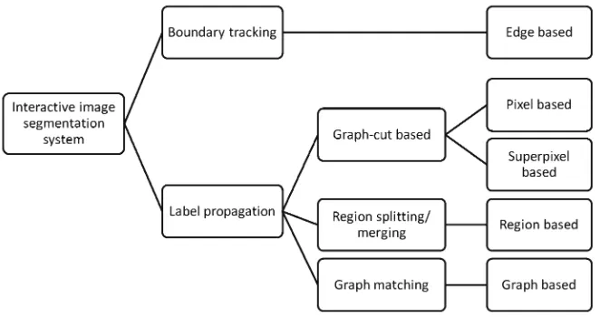
• Boundary Tracking Versus Label Propagation

(22)

2.3 Classification of Solution Techniques 15

Fig. 2.7 Classification of interactive segmentation methods based on interaction types

As an extension, an interactive segmentation system can segment multiple objects at once [8]. It is also possible for an algorithm to conduct the segmentation task on multiple similar images at once [8,27] and even for video segmentation [22]. Fur-thermore, one often encounters 3D (or volumetric) images in the context of medical imaging. Some techniques have been generalized from the 2D to the 3D case for medical image segmentation [21,25]. In this book, we focus on the 2D image seg-mentation.

References

1. Malmberg F (2011) Graph-based methods for interactive image segmentation. Ph.D. thesis, University West

2. Yang W, Cai J, Zheng J, Luo J (2010) User-friendly interactive image segmentation through unified combinatorial user inputs. IEEE Trans Image Process 19(9):2470–2479

3. Grady L (2006) Random walks for image segmentation. IEEE Trans Pattern Anal Mach Intell 28(11):1768–1783

4. Pratt W (2007) Digital image processing: PIKS scientific inside. Wiley-Interscience publica-tion. Hoboken, NJ, USA

5. Koller D, Friedman N (2009) Probabilistic graphical models: principles and techniques. MIT press, Cambridge, MA, USA

6. Li Y, Sun J, Tang CK, Shum HY (2004) Lazy snapping. ACM Trans Graph 23(3):303–308 7. Ning J, Zhang L, Zhang D, Wu C (2010) Interactive image segmentation by maximal similarity

based region merging. Pattern Recogn 43(2):445–456

8. Noma A, Graciano A, Consularo L, Bloch I (2012) Interactive image segmentation by matching attributed relational graphs. Pattern Recogn 45(3):1159–1179

(23)

10. Perez P et al (1998) Markov random fields and images. CWI quarterly 11(4):413–437 11. Boykov Y, Veksler O, Zabih R (1998) Markov random fields with efficient approximations. In:

1998 IEEE computer society conference on computer vision and pattern recognition. IEEE, pp 648–655

12. Boykov Y, Jolly M (2001) Interactive graph cuts for optimal boundary and region segmentation of objects in nd images. In: Eighth IEEE international conference on computer vision, vol 1 2001. IEEE, pp 105–112

13. Rother C, Kolmogorov V, Blake A (2004) “grabcut”: interactive foreground extraction using iterated graph cuts. ACM Trans Graph 23(3):309–314

14. Grady L, Sun Y, Williams J (2006) Three interactive graph-based segmentation methods applied to cardiovascular imaging. In: Paragios N, Chen Y, Faugeras O (eds) Handbook of mathematical models in computer vision, pp 453–469

15. Sommer C, Straehle C, Koethe U, Hamprecht FA (2011) Ilastik: interactive learning and seg-mentation toolkit. In: 8th IEEE international symposium on biomedical imaging (ISBI 2011): pp 230–233

16. Blake A, Rother C, Brown M, Perez P, Torr P (2004) Interactive image segmentation using an adaptive gmmrf model. Comput Vis ECCV 2004:428–441

17. Kim T, Lee K, Lee S (2008) Generative image segmentation using random walks with restart. Comput Vis ECCV 2008:264–275

18. Boykov Y, Veksler O (2006) Graph cuts in vision and graphics: theories and applications. In: Paragios N, Chen Y, Fangeras O (eds) Handbook of mathematical models in computer vision, pp 79–96

19. Vezhnevets V, Konouchine V (2005) Growcut: interactive multi-label nd image segmentation by cellular automata. In: Proceedings of graphicon, pp 150–156

20. Wang J, Cohen MF (2005) An iterative optimization approach for unified image segmentation and matting. In: Tenth IEEE international conference on computer vision, vol 2, ICCV 2005. IEEE, pp 936–943

21. Kass M, Witkin A, Terzopoulos D (1988) Snakes: Active contour models. Int J Comput Vis 1(4):321–331

22. Bai X, Sapiro G (2007) A geodesic framework for fast interactive image and video segmentation and matting. In: IEEE 11th international conference on computer vision, 2007. IEEE, pp 1–8 23. Barrett W, Mortensen E (1997) Interactive live-wire boundary extraction. Med Image Anal

1(4):331–341

24. Mortensen EN, Barrett WA (1995) Intelligent scissors for image composition. In: Proceedings of the 22nd annual conference on computer graphics and interactive techniques, SIGGRAPH ’95. ACM, New York, NY, USA, pp 191–198

25. Boykov Y, Funka-Lea G (2006) Graph cuts and efficient n-d image segmentation. Int J Comput Vis 70(2):109–131

26. Adams R, Bischof L (1994) Seeded region growing. IEEE Trans Pattern Anal Mach Intell 16(6):641–647

(24)

Chapter 3

Interactive Image Segmentation Techniques

Keywords Graph-cut

·

Random walks

·

Active contour

·

Matching attributed rela-tional graph

·

Region merging

·

Matting

Interactive image segmentation techniques are semiautomatic image processing approaches. They are used to track object boundaries and/or propagate labels to other regions by following user guidance so that heterogeneous regions in one image can be separated. User interactions provide the high-level information indicating the “object” and “background” regions. Then, various features such as locations, color intensities, local gradients can be extracted and used to provide the information to separate desired objects from the background. We introduce several interactive image segmentation methods according to different models and used image features.

This chapter is organized as follows. First, we introduce several popular methods based on the common graph-cut model in Sect.3.1. Next, we discuss edge-based, live-wire, and active contour methods that track object boundaries in Sect.3.2, and examine methods that propagate pixel/region labels by random walks in Sect.3.3. Then, image segmentation methods based on clustered regions are investigated in Sect.3.4. Finally, a brief overview of the boundary refinement technique known as matting is offered in Sect.3.5.

3.1 Graph-Cut Methods

Boykov and Jolly [1] first proposed a graph-cut approach for interactive image seg-mentation in 2001. They formulated the interactive segseg-mentation as a maximum a posteriori estimation problem under the Markov random field (MAP-MRF) frame-work [2], and solved the problem for a globally optimal solution by using a fast min-cut/max-flow algorithm [3]. Afterwards, several variants and extensions such

J. He et al.,Interactive Segmentation Techniques, 17 SpringerBriefs in Signal Processing

(25)

18 3 Interactive Image Segmentation Techniques

as GrabCut [4] and Lazy Snapping [5] have been developed to make the graph-cut approach more efficient and easier to use.

3.1.1 Basic Idea

In interactive segmentation, we expect a user to provide hints about objects that are to be segmented out from an input image. In other words, a user provides the information to meet the segmentation objectives. For example, in Boykov and Jolly’s work [1], a user marks certain pixels as either the “object” or the “background,” which are referred to as seeds, to provide hard constraints for the later segmentation task. Then, a graph-cut optimization procedure is performed to obtain a globally optimum solution among all possible segmentations that satisfy these hard constraints. At the same time, boundary and region properties are incorporated in the cost function of the optimization problem, and these properties are viewed as soft constraints for segmentation.

As introduced in Sect.2.2, Boykov et al. [1,7] defined a directional graphG = {V,E}, which consists of a set,V, of nodes (or vertices) and a set, E, of directed edges that connect nodes. In interactive segmentation, user seeded pixels for objects and background are, respectively, represented by source nodesand sink nodet. Each unmarked pixel is associated with a node in the 2D plane. As a result,V consists of two terminal nodes,s andt, and a set of non-terminal nodes in graphG which is denoted byI. We connect selected pairs of nodes with edges and assign each edge a non-negative cost. The edge cost from nodexi and nodexj is denoted asc(xi,xj).

In a directed graph, the edge cost fromxi toxjis in general different from that from

xjtoxi. That is,

c(xi,xj)=c(xj,xi). (3.1)

Figure3.1b shows a simple graph with terminal nodessandt and non-terminal nodesxi andxj.

An edge is called at-link, if it connects a non-terminal node inIto terminal node

t ors. An edge is called an-link, if it connects two non-terminal nodes in I. LetF

be the set ofn-links. One can partitionEinto two subsetsFandE−F [7], where

E−F = {(s,xi), (xj,t),∀xi,xj ∈I}. (3.2)

In Fig.3.1,t-links are shown in black whilen-links are shown in red.

(26)

3.1 Graph-Cut Methods 19

Fig. 3.1 A simple graph example of a 3×3 image, where all nodes are connected to source node

sand sink nodetand edge thickness represents the strength of the connection [6].a3×3 image.

bA graph model for (a).cA cut for (a)

Ford and Fulkerson’s theorem [9] states that minimizing the cut cost is equivalent to maximizing the flow through the graph network from source nodesto sink node

t. The corresponding cut is called a minimum cut. Thus, finding a minimum cut is equivalent to solving the max-flow problem in the graph network. Many algorithms have been developed to solve the min-cut/max-flow problem, e.g., [2, 10]. One may use any of the algorithms to obtain disjoint sets S andT and label all pixels, corresponding to nodes in S, as the “foreground object” and label the remaining pixels, corresponding to nodes inT, as the “background”. Then, the segmentation task is completed.

3.1.2 Interactive Graph-Cut

Boykov and Jolly [1] proposed an interactive graph-cut method, where a user indi-cates the locations of source and sink pixels. The problem was cast in the MAP-MRF framework [2]. A globally optimal solution was derived and solved by a fast min-cut/max-flow algorithm. The energy function is defined as

E(L)=

i∈V

Di(Li)+

(i,j)∈E

Vi,j(Li,Lj), (3.3)

where L = {Li|xi ∈ I}is a binary labeling scheme for image pixels (i.e., Li =0

ifxi is a background pixel andLi =1 ifxi is a foreground object pixel),Di(·)is a

pre-specified likelihood function used to indicate the labeling preference for pixels based on their colors or intensities,Vi,j(·)denotes a boundary cost, and(i,j)∈ E

means thatxi andxj are adjacent nodes connected by edge(xi,xj)in graphG. The

boundary cost,Vi,j, encourages the spatial coherence by penalizing the cases where

adjacent pixels have different labels [8]. Normally, the penalty gets larger, whenxi

andxjare similar in colors or intensities, and it approaches zero when the two pixels

are very different. The similarity betweenxi andxj can be measured in many ways

(27)

Fig. 3.2 Two segmentation results obtained by using the interactive graph-cut algorithm [3,6].

aOriginal image with user markup.bSegmentation result of the flower.cOriginal image with user markup.dSegmentation result of the man

that this type of energy functions, composed of regional and boundary terms, are employed in most graph-based segmentation algorithms.

The interactive graph-cut algorithm often uses a multiplier λ ≥ 0 to specify a relative importance of regional term Di in comparison with boundary term Vi,j.

Thus, we rewrite Eq. (3.3) as:

E(L)=λ·

xi∈I

Di(Li)+

(xi,xj)∈N

Vi,j(Li,Lj). (3.4)

The intensities of marked seed pixels are used to estimate the intensity distributions of foreground objects and background regions, denoted as Pr(I|F)andPr(I|B), respectively. Being motivated by [2], the interactive graph-cut algorithm defines the regional term with negative log-likelihoods in the following form:

DI(Li =1)= −lnPr(I(i)|F), (3.5)

(28)

whereI(i)is the intensity of pixelxi andPr(I(i)|L)can be computed based on the

intensity histogram. The boundary term can be defined as:

Vi,j(Li,Lj)∝ |Li−Lj|exp

−(I(i)−I(j))

2 2σ2

· 1

d(i,j), (3.7)

whered(i,j)is the spatial distance between pixelsxi andxj and the deviation,σ,

is a parameter related to the camera noise level. The similarity of pixelsxi andxj

is computed based on the Gaussian distribution. Finally, the interactive graph-cut algorithm obtains the labeling (or segmentation) resultLby minimizing the energy function in (3.4).

Figure3.2shows two segmentation results of the interactive graph-cut algorithm, where the red strokes indicate foreground objects while the blue strokes mark the background region to model the intensity distributions. Segmentation results are obtained by minimizing the cost function in (3.4).

3.1.3 GrabCut

Rother et al. [4] proposed a GrabCut algorihtm by extending the interactive graph-cut algorithm with an iterative process. GrabCut uses the graph-graph-cut optimization procedure as discussed in Sect.3.1.2at each iteration. It has three main features.

1. GrabCut uses a Gaussian mixture model (GMM) to represent pixel colors (instead of the monochrome histogram model in the interactive graph-cut algo-rithm).

2. GrabCut alternates between object estimation and GMM parameter estimation iteratively while the optimization is done only once in the interactive graph-cut algorithm.

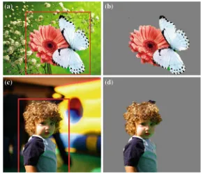
3. GrabCut demands less user interaction. Basically, a user only has to place a rectangle or lasso around an object (instead of detailed strokes) as illustrated in Fig.3.3. A user can still draw strokes for further refinement if needed.

GrabCut processes a color image in the RGB space. It uses GMMs to model the color distributions of the object and background, respectively. Each GMM is trained to be a full-covariance Gaussian mixture with K components. Let k = (k1, . . . ,kn, . . . ,kN),kn ∈ {1, . . . ,K}, where subscriptn denotes the pixel index

andNis the total number of pixels within the marked region. Vectorkassigns each pixel a unique GMM component. The object model and the background model of a pixel with indexn are denoted byαn = 0 and 1, respectively. Then, the energy

function can be written as

E(α,k, θ,z)=U(α,k, θ,z)+V(α,z), (3.8)

(29)

Fig. 3.3 Segmentation results of GrabCut, which requires a user to simply place a rectangle around the object of interest.aOriginal image withrectanglemarkup.bSegmentation result of the flower and butterfly.cOriginal image withrectanglemarkup.dSegmentation result of the kid

θ = {π(α,k), µ(α,k), Σ (α,k)} (3.9)

whereα=0,1,k=1, . . . ,K;πis the mixing weight, andµandΣare the mean and the covariance matrix of a Gaussian component. The data term is given by

U(α,k, θ,z)=

n

D(αn,kn, θn,zn), (3.10)

where

D(αn,kn, θ,zn)= −logπ(αn,kn)+

1

2log|Σ (αn,kn)|

+1

2(zn−µ(αn,kn)])

T_{(Σ (α}

n,kn))−1(zn−µ(αn,kn)) (3.11)

(30)

V(α,z)=γ· (m,n)∈E

Ψ (αn=αm)exp(−β||zm−zn||2), (3.12)

whereΨ (·)is the indicator function that has value 1 if the statement is true and 0, otherwise.

The system first assumes an initial segmentation result by choosing membership vectorskandα. Then, it determines the GMM parameter vectorθby minimizing the energy function in (3.8). Afterwards, with fixed parameter vectorθ, it refines the segmentation resultαand the Gaussian component membershipkby also minimizing the energy function in (3.8). The above two steps are iteratively performed until the system converges.

Rother et al. also proposed a border matting scheme in [4] that refines binary segmentation results to become soft results near the boundary strip of fixed width, where the segmented boundaries are smoother.

3.1.4 Lazy Snapping

Li et al. [5] proposed the Lazy Snapping algorithm as an improvement over the interactive graph-cut scheme in two areas—speed and accuracy.

• To enhance the segmentation speed, Lazy Snapping adopts over-segmented super-pixels to construct a graph so as to reduce the number of nodes in the labeling com-putation. A novel graph-cut formulation is proposed by employing pre-computed image over-segmentation results instead of image pixels. The processing speed is accelerated by about 10 times [5].

• To improve the segmentation accuracy, the watershed algorithm [11], which can locate boundaries in an image well and preserve small differences inside each segment, is used to initialize the over-segmentation in the pre-segmentation stage; it also optimizes the object boundary by maximizing color similarities within the object and gradient magnitudes across the boundary between the object and background.

Figure3.4shows pre-segmented superpixels , which are used as nodes for the min-cut formulation.

After watershed’s pre-segmentation, an image is decomposed into small regions. Each small region corresponds a node in graph G = {V,E}. The location and the color of a node are given by the central position and the average color of the corresponding small region, respectively. The cost function is defined as

E(X)=

i∈V

E1(xi)+λ·

(i,j)∈E

E2(xi,xj), (3.13)

where labelxi takes a binary value (e.g., 1 or 0 if regioni belongs to an object or

(31)

Fig. 3.4 Illustration of the Lazy Snapping algorithm: super-pixels and user strokes (left) and each superpixel being converted to a node in the graph (right). In this example,red strokesstand for the foreground region whileblue strokesdenote the background region. Then, superpixels containing seed pixels are labeled according to their stroke types. The segmentation problem is cast as the labeling of the remaining nodes in the graph.aSuperpixels and user strokes.bGraph with seeded nodes

similarity of nodes andE2(xi,xj)is a penalty term when adjacent nodes are assigned

different labels. The termsE1(xi)andE2(xi,xj)are defined below.

Each node in the graph represents a small region. Furthermore, we can define foreground seedFand background seedBfor some nodes. The colors ofFandB

are computed by the K-means algorithm, and the mean color clusters are denoted by

K_nFandK_mB, respectively. Then, the minimum distance from nodeiwith colorC(i)

to the foreground and background are defined, respectively, as

d_iF =min

n C(i)−K F

n,anddiB=min_m C(i)−KmB. (3.14)

Then, E1(xi)is defined as follows:

⎧

⎪ ⎨

⎪ ⎩

E1(xi =1)=0 and E1(xi =0)= ∞, ifi ∈ F

E1(xi =1)= ∞ and E1(xi =0)=0, ifi ∈ B

E1(xi =1)= dF

i

d_iF+d_iB and E1(xi =0)= dB

i

d_iF+d_iB,otherwise.

(3.15)

The prior energy, E2(xi,xj), defines a penalty term when adjacent nodes are

assigned with different labels. It is in form of

E2(xi,xj)=

|xi−xj|

1+Ci j

(32)

Fig. 3.5 Boundary editing which allows pixel-level refinement on boundaries [5]

whereCi jis the mean color difference between regionsiand j, which is normalized

by the shared boundary length.

Another feature of Lazy Snapping is that it supports boundary editing to achieve pixel-level accuracy as shown in Fig.3.5. It first converts segmented object bound-aries into an editable polygon. Then, it provides two methods for boundary editing:

• Direct vertex editing

It allows users to adjust the shape of the polygon by dragging vertices directly.

• Overriding brush

It enables users to add strokes to replace the polygon.

Then, regions around the polygon can be segmented with pixel-level accuracy using the graph-cut. To achieve this objective, the segmentation problem is formu-lated at the pixel level. The prior energy is redefined using the polygon location as the soft constraint:

E2(xi,xj)=

|xi−xj|

1+(1−β)Ci j +_Dβη2

i j+1

, (3.17)

wherexi is the label for pixeli,Di jis the distance from the center of arc(i,j)to the

polygon,ηis the scale parameter, andβ ∈ [0,1]is used to balance the influence of

Di j. The likelihood energy,E1, is defined in the same way as (3.15). The final

seg-mentation result is generated by minimizing the energy function. Some segseg-mentation examples can be found in [5] and the websitehttp://youtu.be/WoNwNXkenS4.

3.1.5 Geodesic Graph-Cut

(33)

Fig. 3.6 Comparison of segmentation results with the same scribbles as the user input:athe short-cutting problem in the standard graph-cut [6];bthe false boundary problem in the geodesic segmentation [13];cthe geodesic graph-cut [12]; anddthe geodesic confidence map in [12] to weight between the edge finding and the region modeling

Fig.3.6, the geodesic graph-cut algorithm [12] attempts to overcome this problem by utilizing the geodesic distance. It also provides users more freedom to place scribbles. The Euclidean distance between two vertices,xi =(xi1,xi2)andxj =(xj1,xj2), is defined as the l-2 norm of vectorvi,j that connectsxi andxj:

di,j = ||νi,j||2= (xi1−xj1)2+(xi2−xj2)2. (3.18)

The Euclidean distance, which is often used in the graph-cut algorithm, computes the color similarity, e.g., in Eq. (3.7), without taking other properties of pixels along the path into consideration. The geodesic distance between vertices xi andxj is

defined as the lowest cost of the transfering path between them, where the cost between two adjacent pixels may vary depending on several factors. If there is no path connecting verticesxi andxj, the geodesic distance between them is infinite.

The data term in the standard graph-cut algorithm is typically calculated based on the log-likelihood of the color histogram without considering factors such as the locations of object boundaries and seeded points. In contrast, the geodesic graph-cut method uses the geodesic distance as one of the data terms.

Each seed pixel s is either labeled as foreground (F) or background (B). We useΩlto denote the set of labeled seed pixels with labell ∈ {F,B}anddl(xi,xj)

(34)

andΩl. Then,dl(xi,xj)is defined to be the minimum cost among all paths,Cxi,xj,

connectingxi andxj. Mathematically, we have

dl(xi,xj)= min C_xi,_{x j}

1

0

|Wl· ˙Cxi,xj(p)|d p, (3.19)

where Wl are weights along path Cxi,xj. Often, Wl is set to the gradient of the

likelihood that pixelxon this path belongs to the foreground; namely

Wl(x)= ▽Pl(x), (3.20)

where

Pl(x)=

Pr(c(x)|l)

Pr(c(x)|F)+Pr(c(x)|B)

, (3.21)

and wherec(x)is the color of pixelxandPr(c(x)|l)is the probability of colorc(x)

given a color model andΩl. Then, the geodesic distanceDl(xi)of pixelxiis defined

as the smallest geodesic distancedl(s,xi)from pixelxito each seed pixel in form of

Dl(xi)=min s∈Ωl

dl(s,xi). (3.22)

Finally, pixel xi will be labeled with the same label of the nearest seed pixels

measured by the geodesic distance.

Bai et al. [13] extended the above solution to the soft segmentation problem, in which the alpha matte,α(x), for each pixelxis computed explicitly via

α(x)= wF(x)

wF(x)+wB(x)

, (3.23)

where

wl(x)=Dl(x)−r ·Pl(x), l ∈ {F,B}. (3.24)

For the hard segmentation problem, the foreground object hasα =1 while the background region has α = 0. The final segmentation results can be obtained by extracting regions withα=1. Sometimes, a threshold forαis set to extract parts of the translucent boundaries along with solid foreground objects.

There are several other geodesic graph-cut algorithms. For example, based on a similar geodesic distance defined in [13], Criminisi et al. [14] computed the geodesic distance to offer a set of sensible and restricted possible segments, and obtained an optimal segmentation by finding the solution that minimizes the cost energy. Being different from the conventional global energy minimization, Criminisi et al. [14] addressed this problem by finding a local minimum.

(35)

function in Eq. (3.4), the regional term is defined as

Rl(xi)=sl(xi)+Ml(xi)+Gl(xi), (3.25)

wheresl(xi)is a term to represent user stokes,Ml(xi)is a global color model and

Gl(xi)is the geodesic distance defined in Eq. (3.22). Mathematically, we have

MF(xi)=PB(xi), MB(xi)=PF(xi), (3.26)

sF(xi)=

∞,if xi ∈ΩB,

0, Otherwise, (3.27)

and

sB(xi)=

∞,ifxi ∈ΩF,

0, Otherwise. (3.28)

and

Gl(xi)=

Dl(xi)

DF(xi)+DB(xi)

, l ∈ {F,B}, (3.29)

which is normalized by the foreground and background geodesic distance DF(xi)

andDB(xi).

Price et al. [12] redefined this regional term and minimized the cut cost in Eq. (3.4). The overall cost function becomes

E(L)=λR·

i∈V

RLi(xi)+λB·

(i,j)∈E

E2(i,j), (3.30)

whereE2is the same boundary term as that in Eq. (3.16), andλRandλBare

parame-ters used to weight the relative importance of the region and boundary components. A greater value in λR helps reduce the short-cutting problem, which is caused by

a small boundary cost term. For robustness, Price et al. [12] introduced a global weighting parameter to control the estimation error of the color model and two local weighting parameters for the geodesic regional and boundary terms based on the local confidence of geodesic components.

The geodesic graph-cut outperforms the conventional graph-cut [6] and the geo-desic segmentation [13]. It performs well when user interactions separate the fore-ground and backfore-ground color distributions effectively as shown in Fig.3.6.

3.1.6 Graph-Cut with Prior Constraints

(36)

problem by providing shape priors under the min-cut/max-flow optimization frame-work. A shape prior means the prior knowledge of a shape curve template provided by user interaction. Freedman et al. [15] introduced an energy term based on a shape prior by incorporating the distance between the segmented curve,c, and a template curve,c¯, in the energy function as

E =(1−λ)Ei+λEs (3.31)

whereEiis the energy function defined in Eq. (3.4),Esis the energy term associated

with the shape prior, andλis a weight used to balance these two term. Specifically,

Es is in form of

Es =

(i,j)∈E,l_xi=l_{x j}

¯

φ(xi +xj

2 ), (3.32)

wherexiandxj are neighboring pixels in imageI, andlxis the label of pixelx, and

¯

φ(·)is a distance function that all pixelsx on the template curvec¯hasφ(¯ x)= 0. The final segmentation is obtained by minimizing the energy function in Eq. (3.31). Veksler [16] implemented a star shape prior for convex object segmentation. As shown in Fig.3.7, the star shape prior assumes that every single pointxj, which is on

the straight line connecting the center,C0, of the star shape and any pointxi inside

the shape should also be inside the shape. Veksler defined the shape constraint term as

Es =

(xi,xj)∈N

Sxi,xj(li,lj), (3.33)

where

Sxi,xj(li,lj)=

⎧ ⎨

⎩

0, ifli =lj,

∞, ifli =F andlj =B,

β, ifli =B andlj =F,

(3.34)

Fig. 3.7 Astar shapedefined in [16]. Sincered point xiis

inside the object, thegreen point xjon thelineconnecting

xi with centerC0should

(37)

which is used to penalize the assignment of xj with a labellj different from that

of xi. Parameterβ can be set as a negative value, which might encourage the long

extension of the prior shape curve. The final segmentation is the optimal labeling obtained by minimizing the energy function in Eq. (3.31).

Being different from other interactive segmentation methods, a user just provides the center location of a star shape (rather than the strokes for foreground and back-ground regions) in this system. The limitation of the star shape prior [16] is that it only works for star convex objects. To extend this star shape prior to objects of an arbitrary shape, Gulshan et al. [17] implemented multiple star constraints in the graph-cut optimization, and introduced the geodesic convexity to compute the dis-tances from each pixel to the star center using the geodesic distance. We show how the shape constraint improves the result of object segmentation in Fig.3.8.

Another drawback of the standard graph-cut method is that it tends to produce an incomplete segmentation on images with elongated thin objects. Vicente et al. [18] imposed a connectivity prior as a constraint. With additional marks for the dis-connected pixels, their algorithm can modify the optimal object boundary so as to connect marked pixels/regions by calculating the Dijkstra graph cut [18]. This approach allows a user to explicitly specify whether a partition should be connected or disconnected to the main object region.

(38)

Fig. 3.9 Structure of multi-resolution graph-cut [20]. With the segmentation on low-level image, the computation of min-cut on high-level image is highly reduced

3.1.7 Multi-Resolution Graph-Cut

Besides improving the accuracy of the graph-cut segmentation, research has been conducted to increase segmentation efficiency, e.g., reducing the processing time and the memory requirement of a segmentation system (Fig.3.9).

Wang et al. [19] proposed a pre-segmentation scheme based on the mean-shift algorithm to reduce the number of graph nodes in the optimization process, which will be detailed in Sect.3.4.1.2. They also extended the approach to video segmen-tation, and proposed an additional spatiotemporal alpha matting scheme as a post-processing to refine the segmented boundary. To reduce the memory requirement for the processing of high resolution images, Lombaert et al. [20] proposed a scheme that conducts segmentation on a down-sampled input image, and then refines the segmentation result back to the original resolution level (Fig.3.9). The complexity of the resulting algorithm can be near-linear, and the memory requirement is reduced while the segmentation quality can be preserved.

3.1.8 Discussion

(39)

accuracy in some cases. However, there are ways to recover the desired accuracy of object boundaries and object connectivity.

The improvement of the graph-cut based segmentation technique can be pursued along the following directions:

• increasing the processing speed [5,20];

• finding accurate boundary [16,17];

• overcoming the short-cutting problem [12,13].

All of these efforts attempt to achieve a more accurate segmentation result at a faster speed with less user interaction.

3.2 Edge-Based Segmentation Methods

Edge detection techniques transform images into edge images by examining the changes in pixel amplitudes. Thus, one can extract meaningful object boundaries based on detected edges as well as prior knowledge from user interaction. In this section, we present edge-based segmentation methods and show how users can guide the process.

Edges, serving as basic features of an image, reveal the discontinuity of the image amplitude attribution or image texture properties. The location and strength of an edge provide important information of object boundaries and indicate the physical extent of objects in the image [21]. Edge detection refers to the process of identifying and locating sharp discontinuities in an image. It is the key and basic step toward image segmentation problems [22]. In the context of interactive segmentation, many algorithms have been proposed to segment objects of interest based on edge features, combined with user guidance and interaction. Live-wire and active contour are two basic methods that extract objects based on edge features. These two methods will be detailed after an overview on edge detectors.

3.2.1 Edge Detectors

Many edge-detection techniques based on different ideas and tools have been studied, including error minimization, objective function maximization, wavelet transform, morphology, genetic algorithms, neural networks, fuzzy logic, and the Bayesian approach. Among them, the differential-based edge detectors have the longest history, and they can be classified into two types: detection using the first-order derivative and the second-order derivative [22].

(40)

3.2 Edge-Based Segmentation Methods 33

directions while Roberts detectors work better for edges along 45◦and 135◦ direc-tions.

An operator involving only a small neighborhood is sensitive to noise in the image, which may result in inaccurate edge points. This problem can be alleviated by extending the neighborhood size [21]. The Canny edge detector was proposed in [23] to reduce the data amount while preserving the important structural information in an image. There have been a number of extensions of Canny’s edge detector, e.g., [24–26].

The second-order edge detectors employ the spatial second-order differentiation to accentuate edges. The following two second-order derivative methods are popular:

• The Laplacian operator [27]

• The zero crossings of the Laplacian of an image indicate the presence of an edge. Furthermore, the edge direction can be determined during the zero-crossing detec-tion process. The Laplacian of Gaussian (LoG) edge detector was proposed in [28] in which the Gaussian-shaped smoothing is performed before the application of the Laplacian operator.

• The directed second-order derivative operator [29]

• This detector first estimates the edge direction and, then, computes the one-dimensional second-order derivative along the edge direction [29].

For color edge detection, a color image contains not only the luminance infor-mation but also the chrominance inforinfor-mation. Different color space can be used to represent the color information. A comparison of edge detection in RGB, YIQ, HSL and Lab space is given in [30]. Several definitions of a color edge have been exam-ined in [31]. One is that an edge in a color image exists if and only if its luminance representation contains a monochrome edge. This definition ignores discontinuities in hue and saturation. Another one is to consider any of its constituent tristimulus components. A third one is to compute the sum of the magnitude (or the vector sum) of the gradients of all three color components.