www.elsevier.com/locate/dsw
A probabilistic result for the max-cut problem on random graphs
Amir Beck, Marc Teboulle
∗;1School of Mathematical Sciences, Department of Statistic and Operations Research, Tel-Aviv University, Ramat-Aviv 69978, Tel Aviv, Israel
Received 23 June 1999; received in revised form 1 July 2000
Abstract
We consider the max-cut problem on a random graphG with n vertices and weightswij being independent bounded random variables with the same xed positive expectation and variance 2. It is well known that the max-cut number mc(G) always exceeds 1
2
P
i¡jwij. We prove that with probability greater thanpnthe max-cut number satises
1 2
X
i¡j
wij6mc(G)6qn 1
2
X
i¡j wij
!
;
wherepn; qn are explicitly expressed in terms of the problem’s data and such thatpn; qn approach 1 asn→ ∞. c 2000 Elsevier Science B.V. All rights reserved.
Keywords:Probabilistic analysis; Maximum cut; Eigenvalues of random matrices
1. Introduction
Given an undirected graphG= (V; E) with nonneg-ative weightswij=wjion the edges (i; j)∈E, the
max-imum cut problem is that of nding a subset S⊆V
such that P
i∈S; j∈V\Swij is maximized. The
maxi-mum cut ofGwill be denoted by mc(G).
The max-cut problem is of fundamental impor-tance in combinatorial optimization and is known to
∗Corresponding author.
E-mail addresses:[email protected] (A. Amir), teboulle@ math.tau.ac.il (M. Teboulle).
1Partially supported by the Israeli Ministry of Science under Grant No.9636-1-96.
be NP-complete [5]. The max-cut problem also arises in several practical applications. Recently, Goemans and Williamson [7] discovered an approximation al-gorithm for max-cut whose accuracy is signicantly better than all previously known algorithms. This al-gorithm was based on a semi-denite programming relaxation which can be solved approximately in polynomial time. For relevant literature and recent results on the max-cut problem, we refer the reader to Goemans and Williamson [7] and the more recent survey of Goemans [6] and references therein.
It is well known that the max-cut number mc(G) always exceeds 1
2
P
i¡jwij. The main result of this
paper shows that if (wij)i¡jare independent bounded
random variables with the same expectation ¿0 and
variance2 then
with probability greater thanpn, wherepn andqnare
explicitly given and such thatpn; qn→1 asn→ ∞.
To prove our result we rst show in the next section that on any graphGit holds that
1
where min(W) denotes the minimum eigenvalue
of the matrix W = (wij). The last inequality leads
us to investigate the behavior of the ratio rn(W) :=
(1−nmin(W)=2Pi¡jwij)−1, which depends on n
and on the minimum eigenvalue of the matrix W. In Section 3, we show by numerical experiments, that on dierent types of random graphs, the ratiorn(W)
approaches 1 as n gets larger. This is formalized in Section 4 where our main result is presented and ex-plicit expressions forpnandqnare given in terms of
nand the parameter distribution ofW.
2. Bounds for the max-cut
LetG= (V; E) be an undirected graph with vertex setV = 1;2; : : : ; nand nonnegative weightswij=wji
on the edges (i; j)∈Ewithwij= 0; ∀(i; j)6∈E. The
maximum cut ofG consists of nding the setS⊂V
to maximize the weight of the edges with one point in
S and the other point in S:=V \S. To each vertexi, assign the variable xi= 1 if i∈S and−1 otherwise.
Then the problem of nding the weight of the maxi-mum cut can be equivalently written as the following integer quadratic problem:
We will use the following notation. The value of the max-cut problem (M) will be denoted by mc(G). The matrixW= (wij)ni; j=1will stand for the weight matrix
with wij =wji¿0∀i =6 j and wii = 0∀i∈V. The
feasible set of (M) will be denoted by D:={x∈Rn:
x2
i = 1 i= 1; : : : ; n} ≡ {−1;1}n. Recall that for any
symmetric matrix A, the minimum and maximum
eigenvalues denoted, respectively, by min(A) and max(A) satisfy the relations
min(A)6zTAz6max(A) ∀ kzk= 1:
The following result is the starting point of our analy-sis. For completeness we include here a self-contained and easy proof of this result (see also Remark 2.1).
Lemma 2.1. LetG= (V; E)be an undirected graph with a symmetric nonnegative weights matrix W∈Rn×n.Then
Proof. Using our notation we have
mc(G) = max
Now, consider the sum
X
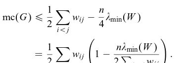
Using this last inequality in (2.1) we thus have
mc(G)61
2
X
i¡j
wij−
n
4min(W)
= 1 2
X
i¡j
wij 1−
nmin(W)
2P
i¡jwij
!
:
The lower bound 12P
i¡jwij is well known in
the literature. The greedy algorithm and local search both nd a cut with value greater than or equal to
1 2
P
i¡jwij. Our interest here is on investigating the
upper bound (1−nmin(W)=2Pi¡jwij)1=2Pi¡jwij
on the max-cut mc(G). By denoting
rn(W) := 1−
nmin(W)
2P
i¡jwij
!−1
;
we see from Lemma 4.1 that ifrn(W) is close to 1 as
ntends to innity then 12P
i¡jwij is a good
approxi-mation for the max-cut for large values ofn. The next section describes numerical experiments showing that
rn(W) is indeed getting close to 1 when n is getting
larger.
Remark 2.1. Eigenvalue bounds and their use in ap-proximating the optimal value of the max-cut mc(G) have been extensively studied in the literature, and we refer the reader to the work of Delorme and Poljak [2] and the survey by Mohar and Poljak [8]. In particular, a better upper bound than the one derived in Lemma 2.1, can be found in [2]. More precisely, it is shown in [2] that mc(G)6’(G) with
(DM) ’(G) = min
u∈Rn
nn
4max(L+ diag(u)):u
Te= 0o;
where L denotes the Laplacian matrix of the graph
G; e is the vector of ones, and diag(u) is the diag-onal matrix with entries ui. In fact, it can be
eas-ily shown that the bound ’(G) is nothing else but thedualbound for problem (M). Moreover, it should be noted that our bound could also be derived from the dual bound ’(G), by choosing the feasible point
u=−We+ (1=n)tr(L)e, where tr(L) is the trace ofL.
Remark 2.2. We would like to emphasize that here
the upper bound derived in Lemma 2.1 is for the sole purpose of deriving a probabilistic analysis of the bound by exploiting powerful properties of
eigenvalues of random symmetric matrices, (see Sec-tion 4). Yet, the numerical experiments given below also show that the simple explicit bound given in Lemma 2.1 already provides for small values ofn a good approximation on the random graphs under con-sideration. The bound’(G), while theoretically bet-ter, requires on the other hand the numerical solution of a dicult non-smooth optimization problem (DM).
3. Behavior ofrn(W): numerical experiments
To understand the behavior of the ratiorn(W) which
depends on the minimum eigenvalue of the matrix
W and n we consider the following experiment on random graphs. We ran 1000 instances on graphs of
nvertices withn= 32;64;128;256;512. We consider 3 types of random graphs when the weights of the matrixW are generated as follows:
TypeA: each weightwij (i ¡ j) is 0 or 1 in
prob-ability 12; and withwii= 0 andwij:=wji (i ¿ j).
TypeB: each weightwij (i ¡ j) is randomly drawn
from the set{0;1;2; : : : ;10}with uniform distribution, and withwii= 0 andwij:=wji(i ¿ j).
TypeC: each weightwij (i ¡ j) is randomly drawn
from the set {0;1;2; : : : ;100} with uniform distribu-tion, and withwii= 0 andwij:=wji (i ¿ j).
We summarize the results of our experiment in Table 1, where we denote by r(G) the ratio rn(W),
and by ˆr(G) its average over 1000 runs. Likewise,
Table 1
Values of ˆr(G) on random graphs
n Type rˆ(G) rmin(G) rmax(G)
A 0.73 0.69 0.77
32 B 0.80 0.77 0.83
C 0.82 0.79 0.84
A 0.79 0.77 0.81
64 B 0.85 0.84 0.87
C 0.86 0.85 0.87
A 0.84 0.83 0.85
128 B 0.89 0.88 0.9
C 0.9 0.89 0.9
A 0.88 0.88 0.89
256 B 0.92 0.92 0.92
C 0.93 0.92 0.93
A 0.91 0.91 0.92
512 B 0.94 0.94 0.94
rmin(G) and rmax(G) denote, respectively, the
mini-mum and maximini-mum values of the ratiorn(W) over the
1000 runs, andndenotes the size of the graph. From the results summarized in Table 1 it can be seen that the ratio ˆr(G) tends to 1 as n gets larger. Another observation is that the rate of convergence de-pends on the way the weights are selected. The above numerical experiments motivate us to theoretically an-alyze the behavior ofrn.
4. Probabilistic analysis of the upper bound
It is known that for unweighted random graphs, the maximum eigenvalue satisesmax(A(G))¿kmin,
wherekmin is the smallest vertex degree in the graph
and A(G) is the adjacency matrix of a graphG, see e.g., [1]. Therefore,max(A(G)) is of magnitude O(n).
A surprising fact is that for a weighted random graph,
min(W) is of magnitude O(n1=2+) for any ¿0
un-der quite general assumptions made on the wayW is randomly generated. This latest fact which was proven by Furedi and Komlos [4] will be a key ingredient in the proof of our main result. More precisely, we need a more specic result tailored to our needs which will be derived from the analysis developed in [4] and is given in Lemma 4.1 below. We rst state our assump-tions and introduce some new notation. The random graph G onn vertices with weights matrixW is as-sumed to satisfy the following conditions:
(C1)Wis ann×nmatrix where the entries (wij)i ¡ j
are independent bounded random variables with the same expectation ¿0 and variance2.
(C2)wij=wji ∀i ¿ jandwii= 0 ∀i.
Lemma 4.1. Let W be a random symmetric
ma-trix satisfying (C1) and (C2), with eigenvalues lambda1(W)¿2(W)¿· · ·¿n(W). Then for any
v¿0and for anyk6(=K)1=3n1=6 we have
Prob
max
26i6n|i(W)|¿2
√
n+v
¡√n
1− v
2√n+v
k
;
whereK∈(0;+∞)is such that|wij−|6K; ∀i ¡ j.
Proof. LetAbe a random symmetric matrix with en-tries aij such that (aij)i6j are independent bounded
random variables with bound K, and with the same expectation= 0 and variance2, and leta
ij=ajifor
i ¿ j. Then, from the claim 3:3 in [4, pp. 237–238, see also p. 236] we have for anyv¿0 andk6(K)1=3n1=6:
Prob
max
16i6n|i(A)|¿2
√
n+v
¡√n
1− v
2√n+v
k
:
LetE be the matrix with all entries 1. Applying the above inequality with the random symmetric matrix
A:=W −E, we thus have
Prob
max
16i6n|i(W −E)|¿2
√
n+v
¡√n
1− v
2√n+v
k
:
To complete the proof, it remains to show that
max
26i6n|i(W)|61max6i6n|i(W −E)|: (4.2)
Noting that
max
26i6n|i(W)|= max{|2(W)|;|min(W)|};
max
16i6n|i(W −E)|= max{|max(W −E)|;
|min(W−E)|}
and using the facts that 2(W)6max(W −E) and min(W)¿min(W−E) (see e.g., Lemmas 1 and 2 in
[4, pp. 237–238]), it can be veried that (4.2) holds, and hence the desired result follows.
We now state and prove our main result.
Theorem 4.1. Let G be a random graph with n
ver-tices and weights matrix W satisfying(C1)and(C2).
Then given∈(0;1
2)and∈(0;1)the following hold: ∀n ¿1with probability greater than
1−√n
1
n+ 1
(=K)1=3n1=6
− 2
2
n(n−1)22; we have
1 2
X
i¡j
wij6mc(G)
61
2
X
i¡j
wij
1 + 2
(1−)
√
n+n1=2+ n−1
Proof. First, by applying Lemma 4.1 with k:=
variables with the same expectation and variance
2. Then, using Tschebyche inequality [3, p. 247],
we obtain that
Hence, in particular, we get
Prob
For convenience, we now dene the following events:
An:={|min(W)|¿2√n+ 2n1=2+};
Combining (4.3) and (4.4) we then obtain
Prob{An∪Bn}6Prob(An) + Prob(Bn)¡1−pn;
denote the complementary events ofAnandBn,
respec-tively. Therefore, with probability greater than pn;
we have obtained that
rn(W) =
where in the rst equality we used the fact that
min(W)60 (since here tr(W) = 0 =Pni=1i(W)¿
nmin(W)), and this completes the proof.
An easy by-product of Theorem 4.1 is the following asymptotic result.
Corollary 4.1. The value of the ratio 12P
i¡jwij=
mc(G) tends to 1 with probability approaching 1
as n → ∞. More precisely, ∀ ¿0; ∃N such that
and hence with probability greater than 1−we have
1 2
P
i¡jwij
Table 2
Values ofpn; andrn;
n pn;1=4 rn;1=4 pn;1=8 rn;1=8 pn;1=16 rn;1=16
100 0.330 0.535 −0:313 0.633 −0:818 0.672
200 0.623 0.588 −0:094 0.698 −0:766 0.740
300 0.729 0.618 0.001 0.733 −0:766 0.740
400 0.788 0.638 0.071 0.756 −0:761 0.797
1000 0.917 0.697 0.320 0.819 −0:661 0.857
5000 0.993 0.784 0.745 0.897 −0:158 0.926
10000 0.998 0.814 0.866 0.920 −0:128 0.945
20000 0.999 0.841 0.940 0.939 0.404 0.959
30000 0.999 0.855 0.966 0.947 0.545 0.966
40000 0.999 0.864 0.978 0.953 0.634 0.970
50000 0.999 0.871 0.984 0.956 0.695 0.973
100000 0.999 0.890 0.995 0.967 0.842 0.980
We note that an asymptotic result similar to the one given in Corollary 4.1 can be found in [2, Theorem 8] where it was established that’(G)=mc(G)→1 as
n→ ∞.
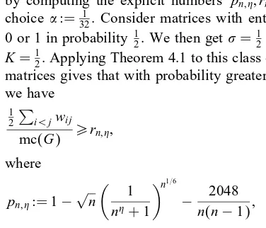
The following example illustrates Theorem 4.1, by computing the explicit numbers pn; ; rn; for the
choice := 1
32. Consider matrices with entries either
0 or 1 in probability 12. We then get=12=12 and
K=12. Applying Theorem 4.1 to this class of random matrices gives that with probability greater thanpn;
we have
1 2
P
i¡jwij
mc(G) ¿rn; ; where
pn; := 1−
√
n
1
n+ 1
n1=6
− 2048
n(n−1);
rn; :=
1
1 + 6431(√n+n1=2+)=(n−1):
Table 2 summarizes the values of the probabilities
pn; and the ratio rn; for various choices of n and
∈(0;1
2). Note that negative values in the probability
columns indicate that the theorem does not furnish any useful information.
References
[1] N.L. Biggs, Algebraic Graph Theory, 2nd Edition, Cambridge University Press, London, 1993.
[2] C. Delorme, S. Poljak, Laplacian eigenvalues and the maximum cut problem, Math. Programming 52 (1991) 481–509.
[3] W. Feller, An introduction to Probability Theory and its Application, Vol. I, Wiley, New York, 1968.
[4] Z. Furedi, J. Komlos, The eigenvalues of random symmetric matrices, Combinatorica 1 (1981) 233–241.
[5] M.R. Garey, D.S. Johnson, Computers and Intractability: A Guide to the Theory of NP-Completeness, Freeman, San Fransisco, CA, 1979.
[6] M.X. Goemans, Semidenite programming in combinatorial optimization, Math. Programming 79 (1997) 143–161. [7] M.X. Goemans, D.P. Williamson, Improved approximation
algorithms for maximum cut and satisability problems using semidenite programming, J. Assoc. Comput. Mach. 42 (1995) 1115–1145.