M – 30
RICE PRICE MODELING IN SIX PROVINCE OF JAVA ISLAND USING
VARMAX MODEL
Nurita Andayani*, I Made Sumertajaya Bogor Agriculture University, Indonesia
Budi Nurani Ruchjana Padjajaran University, Indonesia
Muhammad Nur Aidi
Bogor Agriculture University, Indonesia
*Corresponding email address : [email protected]
Abstract
Rice is an important food commodity in Indonesia because it is not only a main food but also social commodity, and has influence in politic stabilities and economic growth in Indonesia. Based on this condition is showed that everything about rice especially rice price has social economic impact in Indonesia. Factors that influence the domestic rice price in Indonesia are real exchange value, domestic corn price, and basic rice price This research aims to create models of rice price monthly data from six province in Java to real exchange value from 2007 until 2014 by using multivariate time series modeling approach with covariate, that is VARMAX (Vector ARIMAX) model. The results show that rice price in West Java, DI Yogyakarta, and Banten are influenced by rice price in DKI Jakarta, Central Java, and East Java, and real exchange value. Based on RMSE value, the best model is using VECMX(2,1) model.
Keywords : ARIMA, VARMA, VARMAX INTRODUCTION
Rice is an important food commodity in Indonesia because it is not only a main food but also social commodity, and has influence in politic stabilities and economic growth in Indonesia. Based on BPS (Badan Pusat Statistik) data, that measure combination of rice consumption household by Susana’s (National Social Economic Survey) and rice consumption out of household by National Rice Consumption Survey in 2012, Indonesians rice consumption is 114,8 kg each year or 315 gram daily. This consumption is higher than average rice consumption in the world that only 60 kg each year in 2012. Based on this condition is showed that everything about rice especially rice price has social economic impact in Indonesia (Mandei, Katiandagho, Ngangi & Iskandar, 2011). Factors that influence the domestic rice price in Indonesia are real exchange value, domestic corn price, and basic rice price (Malian, Mardianto & Ariani, 2004)
Rice price are observed for several years follow time series data form. Time series is an ordered sequence of observations. Although the ordering is usually trough time, particularly in terms of some equally spaced time intervals, the ordering may also be taken trough other dimensions, such as space. One of models in time series is ARIMA (autoregressive integrated moving average) model. ARIMA model is a univariate time series modeling However, some case is not captured by using ARIMA model only. In order to improve forecasting performance ARIMA model, some case need other explanatory variable and ARIMA model that influenced by other explanatory variable is called ARIMAX model.
development model from Granger (1969) idea. Granger says if there are two variables, x and y have causal relationship where x influence y then the past information of x can predict y. Similar to ARIMA model, if there is other explanatory variable or covariate, then VARIMA model is called VARIMAX model. VARIMAX modeling has been used Ocampo and Rodriguez (2012) and Casals, Hiernaux & Jerez (2010) research. Research by Sa-ngasoongsong, A. (2012) uses Granger Causality to automobile sales modeling using VARMAX model, and the result of his research showed that Granger Causality has advantage to identification and visualization of the causal relationship between the components of automobile sales and economic indicators.
Based on background review, this research aims to create models of rice price monthly data from six province in Java to real exchange value from 2007 until 2014 by using multivariate time series modeling approach with covariate, that is VARMAX (Vector ARIMAX) model. These model are purposed to identification of the causal relationship between rice price in six province, forecasting rice price six province in Java to real exchange value by the best model based on estimation parameter method and VARIMAX form.
RESEARCH METHOD Method and Material
The research uses rice price data in DKI Jakarta, Banten, West Java, Central Java, DI Yogyakarta, and East Java province and real exchange value (rupiah to dollar). Data contains monthly data since January 2007 until December 2014.
Methodology ARIMA Model
ARIMA model is introduced by Box and Jenkins. ARIMA model consist AR (autoregressive) model of order-p, MA (moving average) model of order-q, or combination both, that model is called ARIMA (autoregressive moving average) model. A homogeneous non stationary time series can be reduced to stationary time series by taking a proper degree of differencing (Wei, 2006). ARIMA (autoregressive integrated moving average) model of order (p, d, q) is formed by ARMA model with differencing process. Model ARIMA (p, d, q) can be represented in eq. 1 below :
( ) ( 1− ) ( ) = + ( ) ( ) (1)
where :
( ) : autoregressive operator of order -p ( ) : moving average of order-q
( ) : error
( 1− ) : differencing of order-d
B : backward shift operator = : intercep
Stationarity
If ( ) is a observation in time and ( ) is variable random from stochastic process with random observation sequences ( 1) , ( 2) , …, ( ). A stochastic process is a process that obtained sequence of random variable values to describe data’s behavior in various conditions. A stationary stochastic process gives a stationary time series, and a nonstationary stochastic process gives nonstationary time series. A stationary time series data has three criteria, they are :
2. ( ) =
3. = [ ( ( ) − ) ( ( + ) − ) ]
There are two stationarity in time series, they are stationarity in level and stationarity in variance. Nonstationary time series data in level can be solved by differencing. There are three way to estimate stationarity of time series data :
1. There are trend in graph or time series plot. 2. Using autocorrelation and correlogram coefficient. 3. Unit root test by Augmented Dickey Fuller test.
VARIMAX model
VARIMAX (vector ARIMA with exogenous variable) model is development model from VARIMA model. VARIMAX model is approached multivariate time series data analysis by add to exogenous variable. This model is identic to VAR model in data analysis. VARIMAX model can minimize theory’s approached to catch an economic phenomena. Let
( ) = [ ( 1, ) , ( 2, ) , …, ( , ) ]′, = 1, 2, …,T denote a time series vector of m-
dimensional system. And let ( − ) = [ ( 1, − ) , ( 2, − ) , …, ( , − ) ]′ denote a error vector of m-dimensional system with kth lag model where k = 0, 1, 2, ...,T and ( − ) =
[ ( 1, − ) , ( 2, − ) , …, ( , − ) ]′ denote a covariate (exogeneous variable) vector of m
-dimensional system with ith lag model where i = 0, 1, 2, ...., T. A (p, d, q,)th order of vector ARIMA with sth order of covariate autoregressive, denoted as VARIMAX (p, d, q, s) can represented as shown in eq. (2) below :
( ) = + ∑ ∗ ( − ) + ∑ ( − ) − ∑ ( − ) + ( )
(2) where :
: differencing operator of orde-d.
c : vector of intercept VARIMAX model
: matrix of autoregressive parameter with j lag(j = 1,2, ..., p) : matrix of moving average parameter k lag (k=1, 2, ..., q) ∗ : matrix of parameter with i lag.
VARMAX model can analyze by unrestricted VARMAX and restricted VARMAX. Unrestricted VARMAX is used if time series data is not stationary in level. Time series data must be stationary before using VARMAX model, differencing data is one way solution if data nonstationary. Restricted VARMAX is used if time series data is not stationary but have cointegration. Restricted VARMAX can be used Vector Error Correction Model (VECM) and
Bayesian Vector Error Correction Model (BVECM) approach. In this research, VARIMAX model analyse by SAS 9.3. There are step to analysis data using VARMAX model, they are :
nonstationary data. If data is stationary, we can use Granger Causality to identification and visualization of the causal relationship among variable, and if data is not stationary, we must make cointegration causality test.
2. Estimation parameter. We can estimate parameter VARIMAX model by two method, they are least square and maximum likelihood method. For example,
= [ ( 1) , ( 2) , …, ( ) ] from a zero mean Gaussian N( 0, ) of VARMAX (p, q, s)
process, the log-likelihood function is given by
ln ( , , ∗, | ) = − likelihood function is called maximum likelihood method
3. Diagnostic model. Diagnostic model is used to check assumption in error model. Error model must follow random, independent, and normal distribution ( 0, ) for i variable (where i = 1, 2, ..., m).
4. Forecasting data. Forecasting is a way to predict value in several period ahead. To know, model has a best performance in forecasting, we can use RMSE (root mean square error) value. The smallest RMSE values show the best model.
RESULT AND DISCUSSION
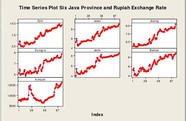
Figure 1. presents time series plot for six Java province and rupiah exchange rate, the figure shows that rice price data for six province and rupiah exchange rate data have upward trend that indicates the data is not stationary in level.
Figure 1. Time series plot of six Java Province and real exchange value
Index
After differencing with lag-1, Dickey Fuller Unit Root Test shows that the null hypothesis can be rejected, that means data do not have unit root or data is stationary (Table 1).
Table 1. Stationary test
Dickey-Fuller Unit Root Tests (Trend) after Differencing
Type Rho Pr <
Rho
Tau Pr < Tau
F Pr > F
Djkt(1) -64.9555 0.0003 -7.37 <.0001 27.43 0.0010
Jabar(1) -63.2355 0.0003 -7.20 <.0001 26.22 0.0010
Jateng(1) -56.3755 0.0003 -6.32 <.0001 20.44 0.0010
Dyogya(1) -71.3994 0.0003 -7.77 <.0001 30.47 0.0010
Jatim(1) -102.967 0.0001 -12.73 <.0001 81.95 0.0010
Banten(1) -72.1254 0.0003 -7.58 <.0001 28.73 0.0010
Kursjual(1) -80.2986 0.0003 -8.22 <.0001 33.77 0.0010
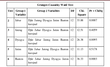
The next step is fixed order ARIMA model, based on AICC values (table 2) show that model AR(2) is best model for rice price data because the value AICC is smallest. Granger causality wald (GC) test (table 3) is used visualization causal relationship among variables. Rice price in DKI Jakarta, Central Java, and East Java cannot be endogenous variables because GC test fail to reject null hypothesis. Based on GC test, three province are become dependent variables in VARMAX model, they are West Java, DI Yogyakarta, and Banten. DKI Jakarta, Central Java, East Java, and Rupiah exchange rate to Dollar are become exogenous variables in VARMAX model
Table 2. Identification first model
Minimum Information Criterion Based on AICC
Lag MA 0 MA 1 MA 2 MA 3
AR 0 61.722216 60.887464 61.005839 61.23494
AR 1 61.090597 60.93515 61.309101 62.043987
AR 2 60.817549 61.295377 62.01877 63.227975
AR 3 61.00556 61.889982 62.836052 64.419931
Table 3. Granger Causality Wald Test
Granger-Causality Wald Test
Test Group 1 Variable
Group 2 Variables DF Chi-Square
Pr > ChiSq
1 Djkt Jabar Jateng Dyogya Jatim Banten kursjual
Granger-Causality Wald Test
Test Group 1 Variable
Group 2 Variables DF Chi-Square
Pr > ChiSq
2 Jabar Djkt Jateng Dyogya Jatim Banten kursjual
12 33.88 0.0007
3 Jateng Djkt Jabar Dyogya Jatim Banten kursjual
12 12.51 0.4059
4 Dyogya Djkt Jabar Jateng Jatim Banten kursjual
12 26.38 0.0095
5 Jatim Djkt Jabar Jateng Dyogya Banten kursjual
12 11.13 0.5178
6 Banten Djkt Jabar Jateng Dyogya Jatim kursjual
12 36.33 0.0003
Based on GC test can shows that rice price in West Java, DI Yogyakarta, and Banten are significant influenced by rice price in DKI Jakarta, Central Java, East Java, and Rupiah exchange rate to Dollar but rice price in DKI Jakarta, Central Java, East Java, and Rupiah exchange rate to Dollar are not influenced by rice price in West Java, DI Yogyakarta, and Banten.
In this research, VARIMAX model is divided two form, unrestricted and restricted VARIMAX model. Restricted form use VECMX model, and this model will compared to unrestricted form. In restricted form, we use Granger causal model to know causal model in VECMX model and the best VECMX model is VECMX(2,1).
Table 4 shows models comparison after models give forecasting to 12 step ahead in three approach, they are unrestricted form of VARIMAX by least square parameter estimation, unrestricted form of VARIMAX by maximum likelihood parameter estimation, and restricted form of VARIMAX by VECMX. Based on smallest RMSE value shows that model VECMX(2,1) gives best model for rice price and real exchange value (table 4). Base on parameter estimation in unrestricted form of VARIMAX, maximum likelihood parameter estimation gives better model than using least square parameter estimation.
Table 4. Model Comparison
Method RMSE (12 step
ahead prediction) VARMAX(2,0,1)Least
Square
379,98
VARMAX(2,0,1)Maximum Likelihood
326,39
VECMX(2,1) 312,45
∆
−0,16047 −0,90799 −0,10900 −0,13126
∆ VARIMAX model, it can be concluded as follows:
1. From the results of Granger causal model, Rice price in West Java, DI Yogyakarta, and Banten are significant influenced by rice price in DKI Jakarta, Central Java, East Java, and real exchange value (Rupiah to Dollar), but rice price in DKI Jakarta, Central Java, East Java, and real exchange value are not significant influenced by rice price in West Java, DI Yogyakarta, and Banten.
2. The best model to forecast rice price in six province of Java Island with real exchange value as covariate is VECMX(2,1). VECMX(2,1) is a restricted form of VARIMAX model, this model give better model than unrestricted form of VARIMAX model by using maximum likelihood and least square parameter estimation method. But model using maximum likelihood to parameter estimation give better model than using least square parameter estimation method.
3. VARIMAX model can be used to model multivariate time series data by adding covariate or exogenous variable, where if we have variable that cannot influenced other variable but this variable can influence other variable.
4. Recently research using VARIMAX model is less then need to further studies if covariat is different among each endogenous variable or covariate is space time data.
REFERENCE
Casals, J., Hiernaux, A. G. & Jerez, M. (2010). From general state space to VARMAX Models.
Granger, C.W.J. (1969). Investigating Causal Relations by Econometric Models and Cross-Spectral Methods. Econometrica, 428-438.
Mandei, J. R., Katiandagho, T., Ngangi, C. R., & Iskandar, J. N. (2011). Penentuan Harga Pokok Beras Di Kecamatan Kotamobagu Timur Kota Kotamobagu. ASE . 7(2) : 15 –21.
Ocampo, S. & Rodriguez, N. (2012). An Introductory Review of a structural VAR-X Estimation and Application. Revista Colombiana de Estadistica. 35(3) : 479-508.
Sa-ngasoongsong, A. (2012). Automobile Sales Modeling using Granger-Causality Graph with PROC VARMAX in SAS(R)9.3. SAS Conference Proceeding : Western Users of SAS Software 2012. California : Long Beach.
Sims, CA. (1980). Macroeconomics and Reality. Econometrica, 48, 1-47.