Urban Poverty?
David Neumark
Scott Adams
a b s t r a c t
Living wage ordinances typically mandate that businesses under contract with a city or, in some cases, receiving assistance from a city, must pay their workers a wage sufficient to support a family financially. We esti-mate the effects of these ordinances on wages, hours, and employment in cities that have adopted such legislation. We then examine the effects of these laws on poverty. Our findings indicate that living wage ordinances boost wages of low-wage workers. Moreover, we find a moderate negative employment effect. Finally, some of the evidence suggests that living wages achieve modest reductions in urban poverty.
I. Introduction
Since December 1994, many cities in the United States have passed living wage ordinances. These ordinances typically mandate that business under con-tract with the city, or in some cases receiving assistance from the city, must pay their workers a wage sufficient to support a family financially. Baltimore was the first city to pass such legislation, and nearly 90 cities have followed suit. Given the increasing popularity of this policy innovation, an empirical investigation of the
ef-David Neumark is Senior Fellow at the Public Policy Institute of California, Professor of Economics at Michigan State University, and a Research Associate of the NBER. Scott Adams is Assistant Professor of Economics at the University of Wisconsin-Milwaukee. This research was partially supported by the Michigan Applied Public Policy Research Funds and the Broad Graduate School of Management, and was completed when Neumark was a Visiting Fellow at the Public Policy Institute of California (PPIC). The views expressed do not reflect those of the Public Policy Institute of California. We thank Jared Bernstein, Robert Pollin, David Reynolds, Peter Schmidt, seminar participants at Harvard, Illi-nois, Missouri, PPIC, Rand, UC-Berkeley, UC-Santa Cruz, and the University of Washington, and anonymous referees for helpful comments. The data used in this article can be obtained beginning Feb-ruary 2004 through January 2007 from David Neumark, Public Policy Institute of California, 500 Washington St., Suite 800, San Francisco, CA 94111.
[Submitted February 2001; accepted November 2001]
ISSN 022-166X2003 by the Board of Regents of the University of Wisconsin System
fects of living wages is in order, to evaluate the claims of beneficial effects made by advocates of these ordinances, and the claims of adverse effects issued by their opponents.1
The feature common to all living wage ordinances is a minimum wage requirement that is higher—and often much higher—than the traditional minimum wages set by state and federal legislation. These wage requirements are typically linked to defini-tions of family poverty. Many ordinances explicitly peg a wage to the level needed for a family to reach the federal poverty line (for example, Milwaukee, San Jose, and St. Paul). Thus, when the federal government defines new poverty lines each year, the living wages in these cities increase. Other localities set an initial wage that is increased annually to take into account increases in the cost of living (for example, Los Angeles and Oakland). Although these latter ordinances may not ex-plicitly state the basis for setting the initial wage, poverty is undoubtedly an underly-ing factor.
Another feature of living wage ordinances is that they are not flexible regarding family size, even though poverty levels vary dramatically depending on the number of children and adults in a household. Similarly, the ordinances do not take account of the income of other family members; for example, if two adults are working for a covered contractor or grantee, both would receive the living wage, placing their incomes well above the poverty level.2 Both of these considerations suggest that
living wage laws may do a poor job of targeting needy families, a criticism also leveled at minimum wages. However, living wage laws may affect a substantially different set of workers than do minimum wages, implying that the effects of living wages on poverty require separate study.
Finally, coverage by living wage ordinances is far from universal. Some cities only impose wage floors on companies under contract with the city (for example, Milwaukee and Boston); this is the most common specification of coverage. Others also impose the wage on companies receiving business assistance from the city (for example, Detroit and Oakland); in almost every case, this is added to coverage of city contractors. Still, other cities also impose the requirement on themselves and pay city employees a living wage (for example, San Jose), although this is less com-mon. This lack of universal coverage also limits the applicability of what is known about the effects of traditional minimum wages—which have near-universal cover-age—to the effects of living wage laws.
To date, there has been no analysis of the actual effects of living wages on the expected beneficiaries—low-wage workers and their families. In this paper, we esti-mate the effects of city living wage ordinances on wages, hours, and employment in cities that have adopted legislation. Most important, we look at the effects of these ordinances on poverty. Given that an increasing number of cities have passed living wage laws recently, and that campaigns for such legislation are under way in numer-ous other cities, it is critical to analyze the effects of these laws on low-wage workers
1. See, for example, http:/ /www.afscme.org/livingwage/, for the claim that living wages reduce poverty, and http:/ /epionline.org/study epi livingwage 08-2000.pdf (p. 29), for the opposite claim.
and poor families.3 Only then can policymakers, employer organizations, labor
unions, and voters make informed judgments regarding the merits of this policy innovation.
Of course a finding that living wage laws reduce poverty would not imply that these laws increase economic welfare overall (or vice versa). Surely someone pays for the higher wages induced by living wage laws, and interpersonal comparisons leading to overall welfare calculations are problematic if not insoluble. In addition, living wage laws, like all tax and transfer schemes, generally entail some inefficien-cies that may reduce welfare relative to the most efficient such scheme. However, it seems rather clear that policymakers and the public regard the poverty rate as an important metric, and living wages as a viable means of attempting to reduce it. Thus, the effect of living wage laws on urban poverty is an important policy issue. If living wage laws fail to reduce urban poverty, the principal argument of living wage advocates would be undermined. But if they achieve this goal, then consider-ations of potential costs of living wages and comparisons with other possible alterna-tives would become quite important.
II. Living Wages and Minimum Wages
Although city living wage ordinances have received little attention from academic researchers, the effects of standard federal or state minimum wages have been studied extensively, both theoretically and empirically. However, there are important reasons why the effects of living wage ordinances may be quite differ-ent. As a result, original research on living wage ordinances is needed to draw reliable conclusions. Nonetheless, the existing work on standard minimum wages provides a useful ‘‘road map’’ for analyzing the consequences of living wage ordinances.
A. Employment Effects
The theoretical predictions regarding the employment effects of minimum wages are well known. Substitution effects act to reduce employment of low-skilled labor, as employers switch from now-more-expensive low-skilled labor toward other in-puts. In addition, assuming firms were minimizing costs initially, the changed input mix raises costs and therefore prices, reducing the overall scale of output as well as input use (‘‘scale effects’’), which also acts to reduce employment of low-skilled labor. The consensus view from earlier time-series studies was that the elasticity of employment of low-skilled (or young) workers with respect to minimum wages was most likely between⫺0.1 and⫺0.2 (Brown, Gilroy, and Kohen 1982). More recent studies have spurred considerable controversy regarding whether or not minimum wages actually reduce employment of low-skilled workers. Although this is not the place to review this evidence (see Neumark and Wascher 1996 for a thorough re-view), a leading economics journal recently published a survey of economists’ views of the best estimates of various economic parameters. Results of this survey—which
was conducted in 1996, after most of the recent research on minimum wages was well known to economists—indicated that the median ‘‘best estimate’’ of the mini-mum wage elasticity for teenagers was⫺0.10, while the mean was⫺0.21 (Fuchs, Krueger, and Poterba 1998). Thus, although there may be some outlying perspec-tives, economists’ views of the effects of the minimum wage are centered on the earlier consensus range.
Living wage ordinances are sure to be binding for some employers with grants or contracts with their city, although quantitative measurement of the fraction of the covered workforce is extremely difficult.4Nonetheless, assuming that some
employ-ers will face higher costs for some workemploy-ers, the predictions of the effects of minimum wages ought to carry over at least qualitatively to the effects of living wages. How-ever, there are at least three unique features of living wages that are likely to weaken their effects, relative to standard minimum wages.
First, the city is a purchaser of goods and services from contractors (and possibly also in an indirect sense from grantees). Thus, it is not necessary that its demand curve for particular services slopes downward, or at least not appreciably over some range. This could be the case either because the city finds it possible to raise taxes to cover higher costs (thus largely allowing contractors to pass through the increased labor costs), or because some services have to be purchased in quantities that may be largely insensitive to price (such as snow plowing). On the other hand, a city government has some limits on its ability to raise taxes. In addition, city contractors or recipients of assistance may pay higher wages to workers who are producing goods and services sold on the private market as well (perhaps the same workers who do some covered work and some uncovered work, or different workers working for the same employer). The responses to wage increases for this work done for the private sector are more likely to be subject to the law of demand.
Second, because living wage laws specify wage levels that must be paid without reference to skill levels of workers, employers who do some work covered by these laws and some work that is not covered may reallocate their skill and higher-wage labor to the former and their lower-skill and lower-higher-wage labor to the latter in order to comply. This may still entail some inefficiencies, but could moderate any cost-increasing effects of living wages.
Third, even under broad definitions of coverage by living wage ordinances, only a fraction of the workforce is likely to be covered, in contrast to the near-universal coverage of minimum wage laws. In this situation, some of the labor disemployed in the covered sector is likely to shift into the uncovered sector. Because wages in that sector can adjust downward in response to the outward supply shift, wages may fall foralllow-skilled workers in that sector, although the state or federal minimum still provides a wage floor that can constrain this response. However, given the wage decline, employment will not expand enough in the uncovered sector to offset fully the employment decline in the covered sector.5
Thus, although the qualitative prediction that higher living wages will adversely affect employment (or hours) of low-skilled workers still stands, there are reasons
4. For an ambitious effort in the context of a proposed living wage ordinance in San Francisco, see Alunan et al. (1999).
to expect the effects to be more moderate than those of minimum wages. Possibly offsetting this in practice, though, is the considerably higher wage floor set by many living wage ordinances.6
B. Distributional Effects
Among the low-skilled workers affected by living wage ordinances, there are likely to be winners and losers. Gains accrue to those whose wages are forced up by the wage requirement, and who retain their jobs (and hours) with covered employers. Workers whose employment prospects worsen, who perhaps end up working at lower-wage jobs in the uncovered sector or nonemployed, lose from living wages. There are some additional possible winners and losers. First, as low-skilled workers disemployed from the covered sector shift to the uncovered sector, wages there may be bid down somewhat, although we suspect that the magnitudes involved are likely to be small. Second, the changes in employment and in the allocation of low-skilled workers across the covered and uncovered sectors could shift relative demands for higher-skilled workers, with the direction of the effects depending, among other things, on whether low- and high-skilled labor are substitutes or complements in production. In addition, there may be wage increases for higher-skill workers attrib-utable to ‘‘ripple’’ effects stemming from increases in the mandated wage floor (Gramlich 1976; Grossman 1983).
Because we have no a priori basis for predicting the full range of effects on work-ers, or whether the workers who lose or benefit are likely to be in higher-income or lower-income families, there are no theoretical predictions for the effects of living wages on poverty. In the minimum wage literature, earlier research speculated that minimum wages would do little to reduce poverty (without addressing the question directly). In particular, it noted that while there are few poor or low-income families with high-wage workers, there are many high-income families with low-wage work-ers (such as teenagwork-ers).7If the job loss tends to be concentrated among low-wage
workers in low-income families, and the wage gains occur more among low-wage workers in higher-income families, minimum wage increases could hurt poor fami-lies or lead to more poor famifami-lies. In fact, recent research using past experiences
6. There are also some possible ‘‘second-round’’ effects of living wage laws. Employers affected by living wage ordinances may in some cases find it more profitable to terminate contracts, grants, tax abatements, etc., with the city. This may reduce the benefits from living wage laws, because those firms most likely to ‘‘select out’’ of city business are those employing the highest shares of low-skilled labor—precisely the workers whom these ordinances are intended to help. In addition, as some firms terminate contracting with the city, fewer firms are left to bid on city contracts, which may—if the number of remaining firms becomes sufficiently small—lead to less competitive bidding and therefore higher prices for city services. Thus, although working out the precise effects of these second-round responses is difficult, it appears most likely that they reinforce the first-round disemployment effects. On the other hand, the decision of some employers to select out of city contracts and grants may increase competition in the private sector, and lower prices there.
with minimum wage increases in the United States finds that a minimum wage does not reduce the proportion of families living in poverty, and if anything instead in-creases it (Neumark, Schweitzer, and Wascher 1998).
This ambiguity in whether minimum wages help poor or low-income families is also apparent in many living wage ordinances. As noted above, the wage require-ments set by these laws frequently impose a wage floor pegged to the federal poverty level for a family with a given number of children, without regard to the income earned by other family members. Thus, there are likely to be at least some beneficia-ries in families whose incomes are well above the poverty line. Nonetheless, because different workers may work in jobs covered by living wage ordinances compared with jobs affected by minimum wages, the distributional effects of living wage laws could easily differ, and there is no a priori reason to rule out living wages being more beneficial than are minimum wages in reducing poverty.
III. Existing Research on the Effects of Living Wage
Ordinances
Because living wage ordinances have been enacted only recently, little empirical research has been conducted on their effects. Most important, no one has attempted a systematic empirical evaluation of the actual (observed) effects of living wage laws on low-wage workers and their families.
The best-known work on living wages is the book by Pollin and Luce (1998, hereafter PL). Although the primary purpose of this book was to advocate living wages as a viable poverty-fighting tool, it is a useful starting point for research on the subject. PL argue that living wage ordinances will deliver a higher standard of living for low-income families. They also posit that such legislation will reduce government subsidy/transfer payments to working families.8This work is
problem-atic. First, PL’s calculations regarding improved living standards and reduced subsidy/transfer payments are based on a family of four in Los Angeles with a single wage earner, despite the facts (given in their book) that (i) only 42 percent of those earning at or below the Los Angeles living wage are the single wage earner in a family, and (ii) the average family size for these workers is 2.1, indicating that on average people potentially affected by living wages are not supporting a family of four. Second, PL do not attempt to estimate whether there are disemployment effects or hours reductions from living wages, but instead assume no such effects. If either results from a living wage increase, then some families may suffer potentially sizable income declines. On the other hand, it is no surprise that calculations based on raising
wages of low-wage workers while assuming no employment or hours reductions will look beneficial to low-wage workers and to some extent to low-income families. In short, PL’s work cannot be viewed as reliable empirical evidence on the effects of living wages on low-income families. Despite this, calculations paralleling PL’s have been used to evaluate proposed ordinances in other cities (for example, Reyn-olds 1999). Not surprisingly, given the assumptions, these evaluations reach similar conclusions.
Other studies have attempted to predict the loss of jobs that will result from living wages. For instance, two studies use existing estimates from the minimum wage literature and apply them to living wages. Tolley, Bernstein, and Lesage (1999) projected that more than 1,300 jobs would be lost in Chicago from the city’s liv-ing wage ordinance. As noted earlier, though, empirical estimates from minimum wage studies may not carry over to living wages. The Employment Policies Institute (1999) estimates that if all of California adopted a living wage, there would be more than 600,000 lost jobs and $8.3 billion in lost income. This calculation assumes that every firm in California would be subject to a living wage law despite the fact that no such state-level laws exist (or are even in the planning stages, to the best of our knowledge). Also, no current ordinance covers all workers. Finally, this calcula-tion assumes that workers who are laid off will not find jobs elsewhere, again ignor-ing the limited coverage of livignor-ing wage laws, which implies the existence of a sub-stantial uncovered sector. Like PL, these studies (and other similar ones) do not attempt to study what has actually happened in localities where living wages have been adopted.
Two studies look at living wage effects following the adoption of legislation, although they focus on the costs of city contracts (Weisbrot and Sforza-Roderick 1996; Niedt et al. 1999). These studies of small numbers of contracts in Baltimore conclude that the real cost of city contracts actually declined as a result of living wage ordinances, thus apparently debunking a central argument of living wage opponents. However, a critique by the Employment Policies Institute (1998) of the study con-ducted by Weisbrot and Sforza-Roderick (1996) questions these results.9In addition,
because these studies focus on one city, there is no ‘‘control sample’’ of cities in which living wages did not increase with which to compare the cost changes for Baltimore.
This brief review emphasizes the need for considerably more analysis of the effects of living wage ordinances on workers and families, studying the actual experiences of cities where living wages have been enacted.10 Proponents of the living wage
make strong claims that poverty will be reduced, and opponents make strong claims that some low-wage workers will lose their jobs as a result of living wages, making poverty increases more likely. Empirical evidence is required to resolve these ques-tions.
9. Among the many problems cited, it is claimed that one of the 23 contracts matched by Weisbrot and Sforza-Roderick was just an extension of a preexisting contract and not subject to the living wage law. Additionally, many contracts considered as post-living wage contracts actually started before the law went into effect. The study claims that correcting these and other errors reverses the findings.
IV. Data on Living Wage Laws and Labor Market
Outcomes
A. Living Wage Laws
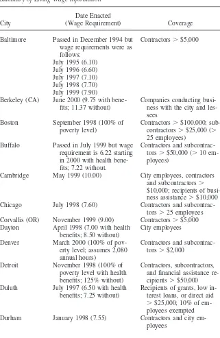
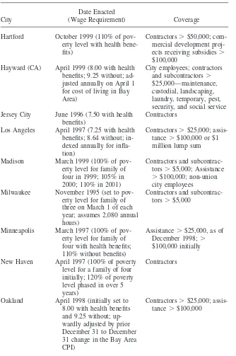
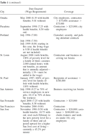
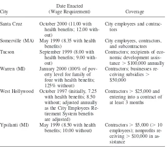
We used multiple sources including personal communications with municipalities to assemble information on living wage ordinances. Although a few laws were passed prior to 1996, most came into effect in 1996 or after. For this reason, and because cities cannot be identified in our data set for a period in 1995, we restrict much of the analysis to 1996 and after.11Table 1 lists information on living wage laws in all
cities, including the wage floors and their effective dates, information on who is covered by these laws, and other details.12This information covers the period through
2000. Not all of these are used in our empirical analysis, as some of the smaller municipalities cannot be identified in our data.13 Because the analysis focuses on
larger metropolitan areas, the failure to identify these municipalities does not con-taminate the control group.14
B. Labor Market Data
The data on labor market outcomes and other worker-related characteristics come from the CPS Outgoing Rotation Group (ORG) files extending from January 1996 through December 2000 and the CPS Annual Demographic Files (ADFs) from 1996 through 2000. The ORG files provide data on wages, employment, hours, etc., for individuals. In these files, residents of all SMSAs, encompassing all large- and me-dium-sized cities in the United States, can be identified. We extract data on these residents for our empirical analysis. In some respects, we would like to know where people work rather than where they live, but such information is not available, and employees of firms covered by living wage laws need not work in the SMSA. Also, the correspondence between cities and SMSAs is imperfect, but because many
11. Specifically, for part of 1995 standard metropolitan statistical area (SMSA) codes are unavailable in the Outgoing Rotation Groups of the Current Population Survey (CPS) due to phasing in of a new CPS sample based on the 1990 Census.
12. Some living wage ordinances specify two different wage floors, one (lower) applicable when health insurance is provided, and another when it is not. We always report results using the lower wage floor applicable when health insurance is provided. The estimates were similar when we re-estimated the models using the higher wage floor.
13. These include Berkeley, Cambridge, Corvallis, Hayward, Pasadena, San Fernando, Santa Cruz, Somer-ville, Warren, West Hollywood, and Ypsilanti. We also cannot identify St. Paul separately in the data, and therefore just apply the Minneapolis living wage (which is nearly identical but came two months later) to the Minneapolis-St. Paul SMSA.
Table 1
Summary of Living Wage Information
Date Enacted
City (Wage Requirement) Coverage
Baltimore Passed in December 1994 but Contractors⬎$5,000
wage requirements were as follows:
July 1995 (6.10) July 1996 (6.60) July 1997 (7.10) July 1998 (7.70) July 1999 (7.90)
Berkeley (CA) June 2000 (9.75 with bene- Companies conducting
busi-fits; 11.37 without) ness with the city and
les-sees
Boston September 1998 (100% of Contractors⬎$100,000;
sub-poverty level) contractors⬎$25,000 (⬎
25 employees)
Buffalo Passed in July 1999 but wage Contractors and
subcontrac-requirement is 6.22 starting tors ⬎$50,000 (⬎10 em-in 2000 with health bene- ployees)
fits; 7.22 without.
Cambridge May 1999 (10.00) City employees, contractors
and subcontractors⬎
$10,000; recipients of busi-ness assistance⬎$10,000
Chicago July 1998 (7.60) Contractors and
subcontrac-tors ⬎25 employees
Corvallis (OR) November 1999 (9.00) Contractors⬎$5,000
Dayton April 1998 (7.00 with health City employees
benefits; 8.50 without)
Denver March 2000 (100% of pov- Contractors and
subcontrac-erty level; assumes 2,080 tors ⬎$2,000 annual hours)
Detroit November 1998 (100% of Contractors, subcontractors,
poverty level with health and financial assistance
re-benefits; 125% without) cipients⬎$50,000
Duluth July 1997 (6.50 with health Recipients of grants, low
in-benefits; 7.25 without) terest loans, or direct aid
⬎$25,000; 10% of em-ployees exempted
Durham January 1998 (7.55) Contractors and city
Table 1(continued)
Date Enacted
City (Wage Requirement) Coverage
Hartford October 1999 (110% of pov- Contractors⬎$50,000;
com-erty level with health bene- mercial development
proj-fits) ects receiving subsidies⬎
$100,000
Hayward (CA) April 1999 (8.00 with health City employees; contractors benefits; 9.25 without; ad- and subcontractors⬎
justed annually on April 1 $25,000—maintenance, for cost of living in Bay custodial, landscaping,
Area) laundry, temporary, pest,
security, and social service
Jersey City June 1996 (7.50 with health Contractors
benefits)
Los Angeles April 1997 (7.25 with health Contractors⬎$25,000; assis-benefits; 8.64 without; in- tance⬎$100,000 or $1 dexed annually for infla- million lump sum tion)
Madison March 1999 (100% of pov- Contractors and
subcontrac-erty level for family of tors ⬎$5,000; Assistance
four in 1999; 105% in ⬎$100,000; non-union
2000; 110% in 2001) city employees
Milwaukee November 1995 (set to pov- Contractors and
subcontrac-erty level for family of tors ⬎$5,000 three on March 1 of each
year; assumes 2,080 annual hours)
Minneapolis March 1997 (100% of pov- Assistance⬎$25,000, as of
erty level for family of December 1998;⬎
four with health benefits; $100,000 initially 110% without benefits)
New Haven April 1997 (100% of poverty Contractors
level for a family of four initially; 120% of poverty level phased in over 5 years)
Oakland April 1998 (initially set to Contractors⬎$25,000;
assis-8.00 with health benefits tance⬎$100,000 and 9.25 without;
Table 1(continued)
Date Enacted
City (Wage Requirement) Coverage
Omaha May 2000 (8.19 with health City employees, contractors
benefits; 9.01 without) ⬎$75,000; assistance⬎
$75,000
Pasadena September 1998 (7.25 with Contractors⬎$25,000; city
health benefits; 8.50 with- employees out)
Portland July 1996 (7.00) Custodial, security, and
park-ing attendant contracts July 1998 (7.50)
July 1999 (8.00; starting in this year, the living wage is 9.00 if health benefits are not included)
St. Louis August 2000 (with benefits, Contractors and business re-130% of poverty level for ceiving tax breaks a family of three; assumes
2,080 annual hours; with-out benefits, an amount that is annually adjusted— initially 1.39—must be added to the wage)
St. Paul January 1997 (100% of pov- Recipients of assistance⬎
erty level for family of $100,000
four with health benefits; 110% without)
San Antonio July 1998 (9.27 to 70% of Business receiving tax breaks service employees in new
jobs; 10.13 to 70% of dura-ble workers)
San Fernando April 2000 (7.25 with health Contractors⬎$25,000 benefits; 8.50 without)
San Francisco November 2000 (9.00) Contractors
San Jose November 1998 (9.50 with Contractors⬎$20,000;
assis-health benefits; 10.75 with- tance⬎$100,000 (ex-out; reset each February to cludes trainees and work-the new poverty level for a ers under 18); city
family of three and ad- employees
Table 1(continued)
Date Enacted
City (Wage Requirement) Coverage
Santa Cruz October 2000 (11.00 with City employees and
contrac-health benefits; 12.00 with- tors out)
Somerville (MA) May 1999 (8.35 with health City employees, contractors,
benefits) and subcontractors
Tucson September 1999 (8.00 with Contractors; recipients of
eco-health benefits; 9.00 with- nomic development
assis-out) tance⬎$100,000 annually
Warren (MI) January 2000 (100% of pov- Contractors; businesses re-erty level for family of ceiving subsidies ⬎
four with health benefits; $50,000 125% without)
West Hollywood October 1997 (initially, 7.25 Contractors⬎$25,000 and with health benefits; 8.50 entering into a contract of without; adjusted annually at least 3 months
as the City Employees Re-tirement System benefits are adjusted)
Ypsilanti (MI) May 1999 (8.50 with health Contractors⬎$5,000 (⬎10 benefits; 10.00 without) employees); nonprofits re-ceiving⬎$10,000 in as-sistance
Note: Some cities are listed in some sources as having living wage ordinances, but instead have prevailing wage laws (for example, New York, Gary, and Memphis). Other cities, like Des Moines, have an average wage goal policy, rather than a living wage law. In addition to the cities in the table, numerous counties and some school districts have adopted similar living wage ordinances. Much of the information for this table was obtained through correspondence with city governments. Some data, however, was obtained through information made publicly available by the Employment Policies Institute (www.epionline.org) and the Association of Community Organizations for Reform Now (www.acorn.org). The consistency of information provided by these two organizations and the city governments gives us confidence in the accuracy and completeness of the above table.
suburban residents may work in the city, this is not necessarily inappropriate.15
Since January 1996, the design of the CPS has resulted in the large- and medium-sized metropolitan areas in the sample being self-representing (Bureau of the Census 1997).16 This is yet another reason for using only information from this
month on.
For several reasons, most of our analysis uses the ORGs, rather than the ADFs.
15. For expositional ease, from this point on we often refer to cities rather than SMSAs.
Table 2
Variables Used in the Analysis
Variable Definition/Construction
CPS ORG variables
Hourly wage Earnings per hour for hourly workers; usual weekly
earnings/usual hours at main job per week for everyone else
Hours worked Usual hours worked per week at main job
Employment Dummy variable set equal to one if individual
cur-rently has a job; set to zero otherwise CPS ADF variables
Total family earnings Sum of annual earnings of each family member Total family income Combined earned and unearned income of each
family member Policy variables
Minimum wage The minimum wage effective in the state in which
the SMSA is located (weighted average of mini-mums if SMSA straddles states)
Living wage The living wage effective in an SMSA
Poverty threshold The yearly income determined by the U.S. Census Bureau below which a family with a given num-ber of adults and children are in poverty Other variables
Year dummy variables Separate dummy variables for each year from 1996 to 2000
Month dummy variables Separate dummy variables for each calendar month (11)
SMSA dummy variables Separate dummy variables for each SMSA
income.17We therefore use the ADFs for the estimates of the effects of living wages
on poverty. The variables constructed from the ORGs and the ADFs, as well as policy variables and other variables used in the regression analysis, are listed and described in Table 2. Their uses in the empirical analysis are described below.
V. Research Design
To infer the wage, hours, employment, and poverty effects of living wage ordinances, changes in outcomes for workers and families in cities passing these ordinances are studied, and compared with changes in outcomes in similar periods for workers and families in a control group of cities not passing such ordi-nances. By looking at changes in outcomes, spurious correlations of living wage laws with unmeasured city-specific factors are avoided. By using cities that do not pass living wage laws as a control group, spurious correlations with changes in out-comes that are common to all cities are avoided. That is, because living wage ordi-nances are not randomly assigned across either space or time, the research design accounts for the possible correlation of living wage laws with unmeasured influences on labor market outcomes that vary across the cities or years in the sample.
We begin the analysis by asking whether there is evidence that living wage laws succeed in boosting wages of low-wage workers. If they do not, of course, then it is unlikely that any positive (or negative) effects will flow from them. This may seem like a trivial question, with the answer certain to be in the affirmative, but indeed there is no research documenting the extent of compliance with these laws.18
In contrast, compliance with standard minimum wage laws has been studied and documented (Ashenfelter and Smith 1979), as have the effects of minimum wages on the wage distribution. A detailed discussion of the specification used to analyze the effects of living wage laws on wages, and of issues that arise in drawing causal inferences from estimates of this specification, is used to provide a more in-depth discussion of the research design that we apply to all of the outcomes that we study. We estimate a wage equation for various ranges of the wage distribution in SMSAs.19Specifically, we look at workers that fall below the 10th percentile,
be-17. Using the ORGs to study family earnings (rather than income) is problematic. Because there is no monthly poverty threshold, one can either choose some arbitrary method of interpolating annual thresholds by month or face differences in poverty rates driven by the month of the year from which monthly data are drawn.
In addition, with the ADFs we are able to obtain one earlier year of data. Because family income information in 1995 is reported in the 1996 ADF, for which SMSA codes are available, information on family income and city of residence for 1995 can also be used in the empirical analysis. Although most living wage activity starts up somewhat later, data from 1995 are useful in the case of living wages in a couple of cities, and for the control group. (But we also report results with the ADFs using the data beginning in 1996, for comparability.)
18. One reason compliance may be an issue is a lag between initial passage of an ordinance and the adoption and dissemination of guidelines to contractors and others, as well as the establishment of an apparatus to verify and enforce compliance. Sander and Lokey (1998) provide case study evidence from Los Angeles indicating slow but increasing progress toward compliance.
tween the 10th and 25th percentiles, between the 25th and 50th percentiles, and between the 50th and 75th percentiles of their city’s wage distribution in a particular month. Pooling data across months, we estimate the following regression for each percentile range
(1) ln(wp
ijst)⫽α⫹Xijstω⫹β ⋅ln(wjstmin)⫹γ ⋅max[ln(wlivjst), ln(wminjst)]
⫹δYYt⫹δMMs⫹δCCj⫹εijst,
wherewpis the hourly wage for individuals in the specified range (p) of the wage
distribution,Xis a vector of individual characteristics,20 wmin is the higher of the
federal or state minimum wage, and wliv is the higher of the living wage or the
minimum wage.21The subscripts i,j,s, and tdenote individual, city, month, and
year.Y,M, andCare vectors of year, month, and city (SMSA) dummy variables.22 ε is a random error term.23 When cities have very few observations for a given
month, determining whether a worker falls in a particular range of the wage distribu-tion is impossible or unreliable. We therefore restrict our sample to workers in city-month cells with at least 25 observations. All SMSAs identified in the CPS and meeting the sample size restrictions are included in the analysis, and hence all of those without living wages but meeting these criteria are used as controls. Each table reports the number of cities used in the analysis.
It is essential to control for minimum wages, because many cities with living wages are in states with high minimum wages, and we want to estimate the indepen-dent effects of living wages. In addition, we have strong expectations that we should see positive wage effects for the lowest-wage workers stemming from minimum wages, so this serves as a check on the validity of the data.
The living wage variable that multipliesγ is specified as the maximum of the (logs of the) living wage and the minimum wage. This imposes the minimum as the wage floor in the absence of a living wage.24 As such, there is no ‘‘qualitative’’
difference associated with the existence of living wages, aside from imposing a higher wage floor. However, because living wages may have different effects from
20. These include controls for age, sex, race, educational attainment, and marital status.
21. In the few cases of SMSAs that straddle states with different minimum wages in some years (Daven-port-Quad Cities, Philadelphia, Portland, and Providence), we use a weighted average of the minimum wages in the two states, weighting by the shares of the SMSA population in each state (averaged over the months of 1996).
22. For all of the specifications reported in the paper, we also estimated less restrictive specifications using unique dummy variables for each month in the sample (so, for example, for two years of data we would have 23 dummy variables instead of one year dummy variable and 11 month dummy variables). The estimates were virtually unchanged.
23. We also estimated the wage equations using the specified wage percentiles for the city (10th, 25th, 50th, and 75th) as dependent variables, rather than the individual-level data on individuals in these ranges. Because we have different numbers of observations per SMSA-month cell, and we expect estimates to be less precise in cells with fewer observations, we weighted by multiplying the observations by (Njst)1⁄2; when
the dependent variable is a percentile for a cell rather than a mean, this is the correct weighting scheme as long as the density is the same across cells (Mood, Graybill, and Boes 1974). The results were very similar to those reported in the paper using individual-level data.
minimum wages, the coefficient is allowed to differ from that of the standard mini-mum wage floor. If living wages boost the wages of low-wage workers, we would expect to find positive estimates ofγwhen we are looking at workers in relatively low ranges of the wage distribution.25 Finally, we also estimate specifications in
which we lagwmin andwlivby six or 12 months, to allow for slower, adaptive
re-sponses to changes in minimum wages and living wages.26
Equation 1 uses a difference-in-differences strategy to identify the effects of living wages. In this framework, the effect of living wages—the treatment—is identified from how changes over time in cities implementing (or raising) living wages differ from changes over the same time period in cities without (or not raising) living wages. This same strategy is used in analyzing the other outcomes (hours, employ-ment, and poverty) considered in this paper. The difference-in-differences strategy is predicated on the assumption that absent the living wage, and aside from differences captured in the other control variables (including city dummy variables), the ment and control groups are comparable. While fixed differences between the treat-ment and control groups are captured in the city dummy variables, potentially more troublesome is a difference in the time pattern of changes stemming, for example, from a different prior trend in a dependent variable in the treatment and control groups. As the specification only includes year and month dummy variables assumed to have the same effects across all observations, such a difference in the time pattern would tend to be incorrectly attributed to the effects of living wages.
To test for different time trends, the sample was restricted to include only the control group and pre-living wage observations on the treatment group. Specifications for each dependent variable were then estimated adding—in addition to the control variables each one includes—a time trend and an interaction between this time trend and a dummy variable for cities later implementing living wages; the living wage variable was dropped because all observations are taken prior to the introduction of a living wage. The estimated coefficient of the time trend interaction provides a test of differential time trends in the treatment and control groups for the dependent variable in question.27In all cases, this estimated coefficient was small and not
sig-nificantly different from zero, which bolsters the validity of the research design.28
25. Among the SMSAs with a living wage effective in a particular month, the living wage was below the 10th percentile in 17.5 percent of cases, between the 10th and 25th percentile in 64.3 percent of cases, between the 25th and 50th percentile in 15.9 percent of cases, and between the 50th and 75th percentile in 2.3 percent of cases.
26. While independence across cities and months in our sample is assumed, it is unlikely that observations on individuals within a given city-month cell are independent. Because of this, the standard errors that would be obtained from estimating Equation 1’s parameters by ordinary least squares are incorrect. We therefore estimate robust standard errors that relax the assumption of independence (and homoscedasticity) within city-month cells. Corrected standard errors are reported in all tables.
VI. Empirical Results
A. Wage Effects
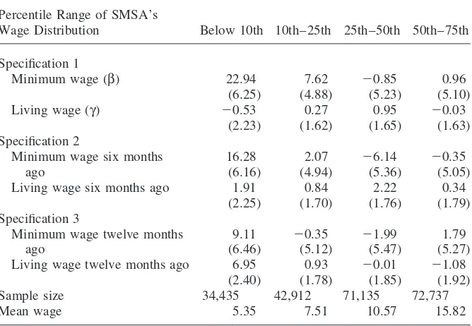
Table 3 reports estimates of the wage equation. Looking first at minimum wages, the estimated wage effects are quite sharp initially for workers below the 10th per-centile. As all coefficient estimates (and standard errors) are multiplied by 100, the estimate implies an elasticity of 0.23. The positive impact between the 10th and 25th percentiles is marginally significant, and no effects show up at higher ranges of the wage distribution. The effects at the lower percentiles dissipate over time. Six months following a minimum wage increase, the estimated elasticity for workers below the 10th percentile falls to 0.16, and after 12 months the estimated elasticity declines to 0.09 and is not statistically significant. At higher ranges of the wage
Table 3
Contemporaneous and Lagged Effects on Log Wages of Workers in Various Percentile Ranges of the Wage Distributions of SMSAs
Percentile Range of SMSA’s
Wage Distribution Below 10th 10th–25th 25th–50th 50th–75th
Specification 1
Minimum wage (β) 22.94 7.62 ⫺0.85 0.96
(6.25) (4.88) (5.23) (5.10)
Living wage (γ) ⫺0.53 0.27 0.95 ⫺0.03
(2.23) (1.62) (1.65) (1.63)
Specification 2
Minimum wage six months 16.28 2.07 ⫺6.14 ⫺0.35
ago (6.16) (4.94) (5.36) (5.05)
Living wage six months ago 1.91 0.84 2.22 0.34
(2.25) (1.70) (1.76) (1.79)
Specification 3
Minimum wage twelve months 9.11 ⫺0.35 ⫺1.99 1.79
ago (6.46) (5.12) (5.47) (5.27)
Living wage twelve months ago 6.95 0.93 ⫺0.01 ⫺1.08
(2.40) (1.78) (1.85) (1.92)
Sample size 34,435 42,912 71,135 72,737
Mean wage 5.35 7.51 10.57 15.82
distribution, all of the estimated minimum wage effects are indistinguishable from zero. This dissipation of the minimum wage effects for low-wage workers is consis-tent with results reported in Neumark, Schweitzer, and Wascher (2004) using a quite different empirical framework. They suggest that this occurs as nominal wages catch up for other workers. Our replication of those results for minimum wages helps to establish the validity of our data set. However, the minimum wage effects are not central here, so in the remaining analyses of wage effects we focus on the impact of living wages.
Table 3 reveals no contemporaneous effects of living wages for the 0th–l0th per-centile range and the 10th–25th perper-centile range. Six months after a living wage increase, the estimated effect for the 0th–10th percentile range is positive, but small and not statistically significant. At a lag of one year, however, we find more strongly significant effects in this range, with an elasticity of 0.07. A lagged effect is not unreasonable. Compliance may well be weaker or slower for living wages than for minimum wages. Moreover, living wage laws are new for most cities in our sample, and implementation of the laws may therefore be a rather drawn-out process, or cities may only enforce compliance as contracts are renewed (as happened, for example, in Baltimore and San Jose). In addition, the smaller elasticity (compared to contempora-neous minimum wage effects) is not surprising, since coverage is much more re-stricted. There is no evidence of a positive impact for workers in the 10th–25th percentile range, or in the higher percentile ranges. The fact that we find no wage effects in higher parts of the wage distribution is evidence against some forms of spurious relationships; that is, one could think of the combined evidence for the different percentile ranges as providing a difference-in-difference-in-differences esti-mate for low-wage relative to high-wage workers. In general, then, these data detect wage-increasing effects of living wage ordinances for the lowest-wage workers, es-pecially about one year after implementation.29
Because in the wage analysis the dependent variable is based on wages falling below a certain level (for the 0th–10th percentile range), there is potential bias from endogenous selection. In particular, focusing on the results for the lowest decile of the wage distribution, some fraction of workers whose wages are raised by a living wage law may be lifted above the 10th percentile cutoff, biasing downward any positive effect of the living wage. As the results ultimately point to a positive effect of living wages on this wage measure, this suggests that the results would only be stronger in the absence of this bias. Note, though, that even if all affected workers have their wage increased to a point above the 10th centile, the average wage of those at or below the 10th centile increases; as low-wage workers are ‘‘cleared out’’ from below the 10th centile, the 10th centile increases, and the bottom 10th of the wage distribution is therefore made up of higher-wage workers on average.30,31
29. We experimented with lags of different lengths. This relationship is relatively robust, with estimated effects strengthening through about one year as the lag is lengthened.
30. To see this in a simple example, suppose there are initially 50 workers, with five earning a wage of $5, 20 earning $6, and 25 earning $7, so the 10th centile is $5. Now let one worker’s wage go from $5 to $7. In this case, the 10th centile rises to $6, and the average wage of workers at or below the 10th centile rises to $5.20.
Nonetheless, the estimates should be interpreted carefully as simply measuring the effect on the average wage of workers whose wages are below the specified cutoff (or within the specified range), rather than measuring a population regression function.32
A natural question is why the minimum wage effects dissipate over time, while the living wage effects do not. Of course given the lags with which living wages increase wages (which, as argued above, is a reasonable expectation), this apparent difference could be solely the result of failure to include longer lags of living wages. Although we do not have a long panel available, we added lags of 18 and 24 months to check this. This resulted in, if anything, slightly stronger positive wage effects of living wages, so the difference seems real. The simplest explanation for this is that the slow process of implementing and enforcing compliance with living wage laws means that the growing effects of these influences may offset any diminution of effects paralleling those that arise with minimum wages. This is especially likely to be true in a short panel that to a large extent captures the beginnings of living wage legislation; data some years down the road should be able to provide more decisive evidence on this question. It is also possible that because many living wage laws are indexed, employers expect the wage constraint to keep pace with inflation, and hence respond differently than to a minimum wage increase.
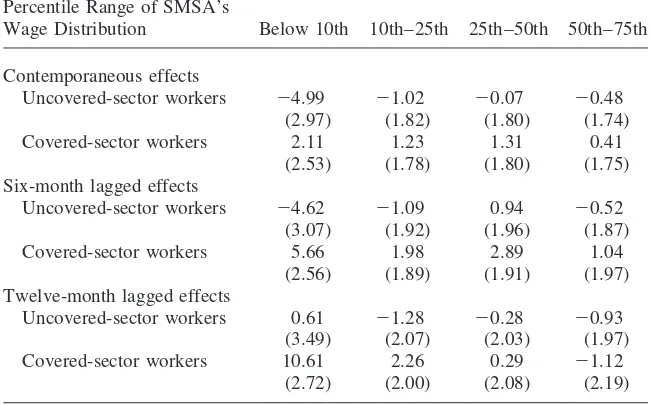
We conduct one additional empirical analysis to try to gauge whether we are truly detecting effects of living wage ordinances, or whether instead the effects we find are spurious. In particular, we attempt to estimate wage effects for workers more likely and less likely to be covered by living wage laws. As discussed earlier, cover-age of living wcover-ages is not universal. Although theory makes no definitive predictions regarding the direction of the effect of living wages on wages of workers in the uncovered sector (see Mincer 1976), we would expect positive effects to be stronger for covered workers, and indeed regard no effect or a negative effect as the most likely outcome for uncovered workers.
Using the limited information we have on workers and the scope of city ordi-nances, we first attempted to identify those individuals who could potentially work for a company under contract with the city, and are therefore potentially covered by their city’s living wage legislation. For workers in cities where businesses receiving financial assistance from the city are covered, virtually any nongovernment worker may work for a company that is subject to the legislation. Therefore, we characterize all private sector workers as being ‘‘potentially covered’’ in these cities. Table 4 details our best attempt at identifying all potentially covered workers, or those who work in the ‘‘covered sector.’’
this empirical strategy would not be viewed as salutary. The analysis of poverty effects that follows, however, speaks to the question of income gains, taking account of wage increases, employment losses, and other changes.
Next, in Equation 1 we replace the living wage variable with a pair of interaction terms—a dummy variable indicating that a worker is potentially covered and a dummy variable indicating noncoverage, each multiplied by the living wage variable. These are intended to reveal the respective effects of living wages on potentially covered and uncovered workers. We also add a series of dummy variables represent-ing the worker subgroups that may be covered by livrepresent-ing wages. Since our estimated definition of potential coverage differs somewhat by city, we had to add separate dummy variables for each group. These dummy variables pick up wage differences between the types of workers that are more likely to be covered, and those that are not, which are separate from any living wage effect but might otherwise be reflected in the interactions with the living wage. The estimates obtained should be interpreted with caution. Some living wage ordinances are not explicit about what types of workers are covered. For many localities, we had to make strong assumptions con-cerning the types of industries in which covered individuals work. Table 4 shows that we chose the broadest definitions of potential coverage, so as not to exclude those that are potentially affected. At best, we identify those workers who could in principle be covered; actual coverage rates should be much lower than those we report. Nonetheless, we suspect that we have probably distinguished between work-ers more and less likely to be covered.
Table 5 reports the results. For workers below the 10th percentile of their city’s wage distribution, those that are identified as potentially covered by legislation ap-pear to experience positive wage effects. These are significant at the 5 percent level when living wages are lagged by 12 months, with an elasticity of 0.11. There are also positive, smaller effects apparent for the contemporaneous and six-month lag, although only the latter is statistically significant. For those unlikely to be covered the evidence points to a negative wage impact if anything, although the estimate falls to zero after 12 months have passed. Wald tests of the equality of coefficients for the 12-month lag specification reveal that the differential effects of legislation on potentially covered and uncovered workers are statistically significant. Overall, although we reiterate the qualification that we only crudely distinguish between cov-ered and uncovcov-ered workers, the results are consistent with those workers more likely to be covered by living wage ordinances receiving the bulk of the wage gains, bolster-ing the case that the effects of livbolster-ing wage laws that we estimate are real; certainly the reverse finding, with stronger wage effects for workers less likely to be covered, would cast doubt on a causal interpretation of the positive overall wage effects re-ported in Table 3.
B. Employment and Hours Effects
limita-The
Journal
of
Human
Resources
Table 4
Summary of the Construction of ‘‘Potentially Covered’’ Worker Variable
Private Industries Classified Public Sector Workers Proportion
as Potentially Covered Classified as in Bottom
Coverage Specified in Legislationa in our Sampleb Potentially Coveredc Quartile
Cities where only contractors are subject to living wage law
Baltimore Contractors⬎$5,000 Construction, transportation — 0.18
(excluding U.S. Postal workers), communica-tions, utilities and sanitary services, custodial, protec-tive service, parking, cer-tain professional and so-cial services
Boston Contractors⬎$100,000; subcontractors Same as Baltimore — 0.20
⬎$25,000
Buffalo Contractors and subcontractors⬎ Same as Baltimore — 0.15
$50,000 (⬎10 employees)
Chicago Contractors and subcontractors (⬎25 Same as Baltimore — 0.18
employees)
Dayton City employees — City employees 0.06
Denver Contractors and subcontractors⬎ Same as Baltimore — 0.17
$2,000
Durham Contractors and city employees Same as Baltimore City employees 0.25
Jersey City Contractors Same as Baltimore — 0.19
Milwaukee Contractors and subcontractors⬎ Same as Baltimore — 0.14
Neumark
and
Adams
511
San Francisco Contractors Same as Baltimore — 0.21
Cities where those receiving business assistance are also subject to living wage law
Detroit Contractors, subcontractors, and finan- All — 0.90
cial assistance recipients⬎$50,000
Hartford Contractors⬎$50,000; commercial de- All — 0.86
velopment projects receiving subsidies
⬎$100,000
Los Angeles Contractors⬎$25,000; assistance⬎ All — 0.90
$100,000 or $1 million lump sum
Minneapolis Assistance⬎$25,000, as of December All — 0.91
1998;⬎$100,000 initially
Omaha City employees, contractors⬎$75,000; All — 0.95
assistance⬎$75,000
St. Louis Contractors and businesses receiving tax All — 0.90
breaks
San Antonio Businesses receiving tax breaks All — 0.86
San Jose Contractors⬎$20,000; assistance⬎ All (excluding workers un- City employees 0.94
$100,000 (excludes trainees and work- der 18)
ers under 18); city employees
Tucson Contractors; recipients of economic de- All — 0.82
velopment assistance⬎$100,000
an-nually
Note: Only information for those cities that are large enough to make our sample cut for the wage analysis in Table 3 are included in this table. a. The ‘‘Coverage specified in legislation’’ column repeats information from Table 1.
b. Three-digit industry codes in the CPS were used to identify non-public sector workers that were most likely subject to living wage legislation. ‘‘Certain professional and social services’’ include health services, libraries, educational services, job training, child care, family care, residential care, miscellaneous social services, museums, architectural and surveying, accounting and auditing, research and testing, management and public relations, and miscellaneous professional and related services. This is based on a study of Baltimore’s living wage law (Niedt, et al., 1999) that looked at the types of workers and firms with city contracts.
Table 5
Contemporaneous and Lagged Living Wage Effects on Log Wages of Covered Sector and Uncovered Sector Workers in Various Percentile Ranges of the Wage Distributions of SMSAs
Percentile Range of SMSA’s
Wage Distribution Below 10th 10th–25th 25th–50th 50th–75th
Contemporaneous effects
Uncovered-sector workers ⫺4.99 ⫺1.02 ⫺0.07 ⫺0.48
(2.97) (1.82) (1.80) (1.74)
Covered-sector workers 2.11 1.23 1.31 0.41
(2.53) (1.78) (1.80) (1.75)
Six-month lagged effects
Uncovered-sector workers ⫺4.62 ⫺1.09 0.94 ⫺0.52
(3.07) (1.92) (1.96) (1.87)
Covered-sector workers 5.66 1.98 2.89 1.04
(2.56) (1.89) (1.91) (1.97)
Twelve-month lagged effects
Uncovered-sector workers 0.61 ⫺1.28 ⫺0.28 ⫺0.93
(3.49) (2.07) (2.03) (1.97)
Covered-sector workers 10.61 2.26 0.29 ⫺1.12
(2.72) (2.00) (2.08) (2.19)
Note: See Table 3 notes for details.
tions, imputing wages for everyone in the sample, and using percentiles of the im-puted wage distribution for our cutoffs.33
Results are reported for employment in Table 6. Turning first to the minimum wage, there is no clear evidence of either positive or negative effects.34The
employ-ment analysis for living wages points to negative effects in all three specifications
33. We obtain the predicted wage in the same manner described in the previous footnote. We use predicted wages for all respondents, whether or not they work, because if we used actual wages for workers and imputed wages for nonworkers we would rarely have nonworkers in the extreme percentiles of the wage distribution. Another alternative is to use the actual wage for workers and a predicted wage plus a randomly generated residual for nonworkers. But this would imply asymmetric treatment of the observations based on the dependent variable, with more accurate classification for those holding a job. Finally, trying to infer something about residuals for nonworkers based on their decision not to work requires identification of a selection model, which we think is tenuous. However, we would expect the market wages faced by those who choose not to work to be on average lower than those faced by observationally equivalent individuals who choose to work (paralleling the standard sample selection problem). To assess the consequences of this in a simple manner, the estimates were recalculated reducing the predicted wages of the nonworkers by 5 percent and 10 percent. The results were similar.
Table 6
Contemporaneous and Lagged Effects on the Probability of Employment in Various Ranges of the Imputed Wage Distributions of SMSAs
Percentile Range of SMSA’s
Imputed Wage Distribution Below 10th 10th–25th 25th–50th 50th–75th
Specification 1
Minimum wage ⫺1.25 7.19 3.21 ⫺1.79
(5.94) (5.12) (3.69) (3.17)
Living wage ⫺1.77 0.02 2.58 1.79
(2.14) (1.81) (1.18) (1.04)
Specification 2
Minimum wage six months 2.33 6.86 0.65 ⫺0.09
ago (6.05) (5.08) (3.66) (3.18)
Living wage six months ago ⫺3.22 1.16 2.31 1.32
(2.26) (1.88) (1.24) (1.08)
Specification 3
Minimum wage twelve 8.05 ⫺0.24 6.96 ⫺3.17
months ago (6.29) (5.20) (3.74) (3.23)
Living wage twelve months ⫺5.62 1.62 1.55 2.44
ago (2.45) (2.02) (1.31) (1.16)
Sample size 83,326 118,541 197,477 199,703
Mean percentage employed 43.98 58.70 68.80 79.12
Note: Reported are the estimated effects of the minimum wage and living wage effective in an SMSA on the employment of individuals in the ranges of the imputed wage distribution in SMSA-month cells specified at the top of each column, using linear probability models. All estimates are multiplied by 100. Because the living wage is expressed in logs, elasticities are given by the coefficient divided by the mean percentage reported in the last row of the corresponding column. The wage distribution is imputed using basic respon-dent characteristics described in the text. Observations for which allocated information is required to con-struct the employment variable in the CPS are dropped. A total of 223 cities are used in the analysis. See Table 3 notes for further details.
for the lowest-wage workers. The effect is statistically significant in the 12-month lag specification, precisely where the significant positive wage effect showed up. The estimates imply that a 10 percent increase in the living wage lowers the probability of employment by 0.0056.35Since 44 percent of those in this imputed wage category
are employed (last row of table), this estimated effect represents an elasticity of
⫺0.13 (5.6/44), evaluated at the mean. Thus, the estimated disemployment effect appears moderate, although account should be taken of the fact that living wage laws do not cover many workers. There is some evidence of positive employment
effects for workers in the higher percentiles of the wage distribution, which could be attributable to substitution. The evidence of employment reductions among low-skilled workers stemming from living wages will work against the positive effects on wages reported earlier, when we look at effects on poverty. In looking at hours, we found no evidence of sizable or statistically significant effects of living wages for those at the lower end of the predicted wage distribution, although the point estimates were negative.36Thus, only for employment is there evidence of adverse
effects of living wages.
C. Poverty Effects
Finally, the central question in evaluating the policy effectiveness of living wage laws is whether they help families escape poverty. We consider two related questions. First, as suggested in the introduction, living wage laws are designed to help families earn their way out of poverty. Thus, we first ask whether living wage laws increase the probability that families’ earnings exceed the poverty line. Note that the resulting definition of poverty does not correspond to the ‘‘official’’ definition, because we use data on earnings only, and not unearned income, transfers, etc.37Nonetheless,
the impact of living wages on the ability of families to earn their way out of poverty is an important policy question, as policies that accomplish such goals via earnings rather than transfers tend to attract more political support (for example, the EITC versus AFDC). Following that, we turn to a parallel analysis using total family in-come. If fighting poverty is the goal of living wages, these estimates are more appro-priate than the estimates obtained using just total family earnings. Not only do they take into account both the gains in family earnings that result from living wages as wages of family members increase, and the declines in family earnings that result when employment or hours are reduced by the legislation, but they also take into account differences in transfer income or other income received as a result of the changing wages, hours, or employment status of family members. As noted earlier, for these analyses we use the (March) ADF files of the CPS.38
In both cases, we compute whether a family’s earnings or income are below the poverty line (denoted by P), and estimate the following equation
(2) Pijt⫽α⫹β ⋅ln(wmin
jt )⫹γ ⋅max[ln(wlivjt), ln(wminjt )]
⫹δYYt⫹δCCj⫹εijt.
We begin, in Table 7, using the 1997–2000 ADFs, which contain information on family earnings and incomes from 1996–99. This corresponds as closely as possible to the years covered by the ORG data.39However, because the ADF covers all
indi-36. These results are not reported in the tables, but are available from the authors upon request. 37. In this analysis we exclude families with members aged 65 years or older. Because of Social Security, those who are at least 65 are more likely to have substantially greater income than earnings.
38. We treated related subfamilies as distinct families for the analysis reported in the paper. The results were qualitatively similar but a bit weaker statistically when we combined related subfamilies and primary families.
viduals in the sample in March, rather than one-fourth (as in the ORGs), there is a larger set of SMSAs for which we have at least 25 observations.
Column 1 presents the estimates of the effects of living wages and minimum wages on poverty based on earnings alone.40The estimated living wage effects are
consistent with living wages reducing poverty, as the estimates for the contempora-neous, six-month, and 12-month lag specifications are negative and significant. The estimates are stronger the longer the lag, consistent with the pattern of estimated wage effects (although the negative employment effects also strengthened with the lag length). In Column 2 we use the larger sample, adding data from 1995 (for which identifying SMSAs in the ADF is not problematic, unlike the ORGs). This results in the estimated coefficients falling in absolute value, while remaining negative and generally significant.
Columns 3 and 4 turn to the analysis of living wage legislation and poverty based on total family income. In both columns, the estimated effects of living wages on the probability that a family is poor are always negative, but statistically significant (at the 5 percent or 10 percent level) only in the 12-month lag specification.41The
estimates for the effects of living wages using total income to classify families as poor indicate that a 10 percent increase in the living wage reduces the probability that a family lives in poverty by 0.0033 to 0.0039. The implied elasticity is about
⫺0.19.
It is worth considering whether the estimated effects on poverty are plausible, given the magnitudes of the wage effects noted earlier indicating that a similar 10 percent increase in the living wage boosts average wages of low-wage workers by only 0.7 percentage point. Of course no one is claiming that living wages lift a family from well below the poverty line to well above it. But living wages may help nudge some families over the poverty line, especially when we recognize that this estimated wage impact is an average effect, whereas the more likely scenario is larger gains concentrated on fewer workers and families. For example, if the 0.7 percentage point average wage increase is concentrated on 10 percent of low-wage workers (1 percent of workers overall), then the implied wage increase for them is 7 percent. If we consider a worker earning the federal minimum, this translates into an earnings in-crease of $720 over the course of the year for a full-time worker; for a higher-wage worker the annual earnings increase would of course be larger. If the families of one-third of the affected workers (0.33 percent of all families) are initially poor and are lifted above poverty, then the reduction of poverty would approximately equal the magnitudes implied by the poverty estimates noted in the previous paragraph; while one third may seem high, earnings gains of $800 or $900 or more are not out of the question. Thus, even coupled with some employment reductions, if a fair
40. Since the ADFs contain earnings and income information from the prior calender year, the estimated effects of the December living wage, the June living wage, and the January living wage, correspond roughly to the effect of the contemporaneous living wage, the living wage sixth months ago, and the living wage 12 months ago in the ORGs, respectively. The same is true of minimum wages. Estimates were also obtained using a weighted average of the applicable minimum and living wage in the SMSA over the year. As might be expected, the estimated effects were quite close to the estimated effects using the June (mid-year) minimum wage and living wage.
The
Journal
of
Human
Resources
Table 7
Contemporaneous and Lagged Effects on the Probability that Family Earnings or Income Fall Below the Poverty Line
Using Urban Workers in Same State as Control Group
Based on Total Based on Total Based on Based on
Earnings Incomea Total Earnings Total Income
(1) (2) (3) (4) (5) (6)
Specification 1
Minimum wage (December) ⫺7.29 ⫺2.18 ⫺13.77 ⫺9.09 ⫺2.56 ⫺9.18
(6.27) (4.84) (7.08) (5.44) (4.83) (5.45)
Living wage (December) ⫺3.27 ⫺2.20 ⫺0.61 ⫺0.03 ⫺2.71 ⫺0.16
(1.45) (1.31) (1.60) (1.46) (1.43) (1.56)
Specification 2
Minimum wage six months ago ⫺1.03 3.44 ⫺8.39 ⫺3.30 3.04 ⫺5.21
Neumark
and
Adams
517
Specification 3
Minimum wage twelve months ago ⫺5.54 ⫺2.07 ⫺3.54 ⫺0.28 ⫺2.31 ⫺0.33
( January) (5.33) (4.78) (6.58) (5.86) (4.77) (5.84)
Living wage twelve months ago ⫺5.08 ⫺4.84 ⫺3.85 ⫺3.34 ⫺5.47 ⫺3.45
( January) (1.44) (1.35) (1.76) (1.73) (1.55) (1.78)
Years that sample covers 96–99 95–99 96–99 95–99 95–99 95–99
Number of observations 107,821 134,584 82,195 103,601 134,584 103,601
Mean percentage below poverty 25.78 26.01 18.62 18.73 26.01 18.73
Note: Reported are the estimated effects of minimum wages and living wages effective in an SMSA on whether a family’s earnings or income are below the poverty line, using linear probability models. All estimates are multiplied by 100. Because the living wage is expressed in logs, elasticities are given by the coefficient divided by the mean percentage reported in the last row of the corresponding column. Given that the ADF surveys are conducted in March and information on family earnings and income refer to the prior calendar year, the applicable contemporaneous and lagged minimum and living wages are noted in parentheses in the left-hand column. The regressions include only year dummy variables, and not the month dummy variables included when using the ORGs in earlier tables. Observations for which allocated information is required to construct the total earnings variable or the total income variable in the CPS are dropped for the relevant analyses. A total of 229 cities are used in the earnings analysis and 218 are used in the income analysis. See Table 3 notes for further details.