Numerical Modeling of Turbulent Bottom Boundary Layer over Rough Bed under Irregular Waves

Numerical Modeling

of Turbulent Bottom Boundary Layer

over Rough Bed under Irregular Waves

Taufiqur Rachman1, Suntoyo2, Kriyo Sambodho2, Haryo Dwito Armono2, and Eko Yusroni3

AbstractAnumerical modelof turbulent bottom boundary layer over rough bed under irregular waves is reviewed. The turbulence model is based upon Shear Stress Transport (SST) k- model. The non-linear governing equations of the boundary layer for each turbulence models were solved by using a Crank-Nicolson type implicit finite-difference scheme. Typical the main velocity distribution, turbulence kinetic energy and time series of the bottom shear stress are presented. These results are shown to be in generally good agreement with experimental result. The roughness effects in the properties of turbulent bottom boundary layer for irregular waves are also presented with several values of the roughness parameter (am/ks) from am/ks=5 to am/ks=3122. The roughness effect tends to decrease the main velocity distribution and to increase the turbulent kinetic energy in the inner boundary layer, whereas in the outer boundary layer, the roughness alters the mean velocity distribution and the kinetic energy turbulent is relatively unaffected. The effect of bed roughness on the bottom shear stress under irregular waves is found that the higher roughness elements increase the magnitude of bottom shear stress along wave cycle. And further, the bottom shear stress under irregular waves is examined with the existing calculation method and the newly proposed method.

Keywordsbottom shear stress, irregular wave, rough bed, turbulent bottom boundary layer

AbstrakDitinjau sebuah model numerik turbulent bottom boundary layer melalui dasar kasar pada gelombang irreguler. Model turbulen didasarkan pada model Shear Stress Transport (SST) k-. Persamaan-persamaan tidak linier boundary layer untuk model turbulen diselesaikan secara numerik dengan menggunakan Crank-Nicolson type implicit finite-difference scheme.Disajikan pula tipikal distribusi kecepatan rata-rata, energi kinetik turbulen dan variasi waktu tegangan geser dasar. Hasil ini secara umum menunjukkan kesesuaian yang baik dengan hasil eksperimen. Pengaruh kekasaran dalam properti turbulent bottom boundary layer untuk gelombang irreguler juga disajikan dengan beberapa nilai parameter kekasaran (am/ks) dari am/ks=5 hingga am/ks=3122. Efek kekasaran cenderung menurunkan distribusi kecepatan rata-rata dan meningkatkan energi kinetik turbulen di dalam boundary layer, sementara di luar boundary layer, perubahan kekasaran terhadap distribusi kecepatan rata-rata dan energi kinetik turbulen relatif tidak terpengaruh. Efek kekasaran pada tegangan geser dasar untuk gelombang irreguler menunjukkan bahwa elemen kekasaran lebih tinggi akan meningkatkan besaran tegangan geser dasar sepanjang siklusgelombang.Lebih lanjut, tegangangeser dasar pada gelombang irreguler diuji dengan metode perhitungan yang ada dan suatu usulan metode baru.

Kata Kuncitegangan geser dasar, gelombang irreguler, dasar kasar, bottom boundary layer

I.INTRODUCTION1

n understanding of nature of the wave boundary layer above the seabed is of fundamental importance to coastal engineers and workers in the field of sediment transport. A number of experimental studies have made new contributions to our understanding of the turbulent behavior of oscillatory flow over both smooth and rough boundaries [1-4]. From these studies, it is clear that turbulence is generated in the vicinity of near-bed regions either through shear layer instability or the turbulence bursting phenomenon.

One problem encountered in the experimental investigation of the wave boundary layer is that it is very thin, of the order of 0-5 cm. In the laboratory, it is usually difficult to get the boundary layer turbulent in the

1

Taufiqur Rachman is with Department of Ocean Engineering, Engineering Faculty, Hasanuddin University, Makassar, 90245, Indonesia. E-mail: ocean_d321@yahoo.com.

Suntoyo, Kriyo Sambodho and Haryo Dwito Armono are with Department of Ocean Engineering, FTK, Institut Teknologi Sepuluh November, Surabaya, 60111, Indonesia. E-mail: suntoyo@oe.its.ac.id.

Eko Yusroni is a Graduated Bachelor Student of Ocean Engineering Department, FTK, Institut Teknologi Sepuluh November, Surabaya, 60111, Indonesia.

.

ordinary. For this reason, the wave boundary layer is quite often studied in an oscillatory tunnel where much larger near-bed orbital velocities can be obtained. Examples of such tunnels are the oscillating water tunnel [4-6] and the oscillating wind tunnel [2, 7-8]. Since is difficult to make controlled field measurement in this thin layer, various analytical and numerical models have been developed in recent. These have been concerned principally with the determination of the velocity and shear stress fields in the oscillatory turbulent boundary layer beneath surface waves. The results have been used to quantify, e.g. the wave drag coefficient, boundary layer thickness and phase lead of the bottom shear stress over the oscillating free stream flow [7, 9-10]. These results have been in turn to compute energy dissipation rates and to estimate sediment transport rates, see e.g. in [11-13].

irregular wave show satisfactory result when compared with input spectral properties. Model results have been compared with experiment data and an excellent agreement has been obtained. Moreover, an experimental and numerical study has been conducted by [10] to investigate the properties of irregular wave boundary layers on a rough bottom. The triangular elements, similar to those used by [1], were pasted on the bottom surface as roughness. It was observe that the turbulence might persist under a free-stream Reynolds numbers within laminar range. The original version of

k- model and two versions of two-layer k- models have been used to predict the boundary layer properties under experimental conditions. It was found that the model could reproduce the shear stress variation in time quite successfully but the magnitude could not be predicted adequately.

Recently, the wave boundary layers over a stone-covered bed with a rather small roughness parameter have investigated by [15]. The outcomes show that the turbulent boundary layer is not extremely sensitive to the packing pattern, the packing density, the number of layers, or the surface roughness of the roughness element. The outcomes further show, the friction factor for small values in the range of am/ks=0.6-3.0 is not a

constant value, which is contrary to suggestions of some previous investigators.

More recently, the characteristics of turbulent boundary layer under saw-tooth waves over rough bed through laboratory and numerical experiments have presented by [12]. A good agreement between numerical and experiment data for mean velocity distribution, turbulent intensity and bottom shear stress was obtained. The effect of roughness on the turbulent boundary layers under asymmetric wave has investigated by [13] using the BSL k- turbulence model validated with experimental data. The BSL k- model could predict well the mean velocity, turbulent intensity and kinetic energy, and bottom shear stress for asymmetric waves. The boundary layers characteristics for laminar, transition and turbulent flow regimes under solitary wave are investigated by [16] using two equations of the Base Line (BSL) k-turbulent model. The model is examined by the linearized boundary layer equations of motion velocity profile in the laminar boundary layer in spatial variation and which is converted to temporal variation. Hydrodynamic conditions were examined subsequently and interpreted using methods comprising turbulent kinetic energy, velocity profile distribution, bottom shear stress, phase difference and friction factor methods. And further, a conduit water tunnel with a downstream gate has been newly proposed to investigate boundary layer characteristics under solitary wave over smooth bed [17]. The generation system presented in this study facilitates measurements of statistical properties obtained by phase ensemble averaging. Validations of the system have been done in terms of free stream velocity, single and periodical oscillatory motion measurements and also time variation of velocity distribution. The critical Reynolds number obtained from this study shows good

agreement with the finding of previous researchers.

The purpose of this paper is to applied a theory describing one of the two-equation turbulence models, Shear Stress Transport (SST) k- model, proposed by

[18] in a rough turbulent boundary layer to compute turbulent boundary layer properties through numerical methods. The numerical results are verified through experimental data by [19]. Typical vertical profiles of horizontal velocity, turbulence energy and eddy viscosity, and time series of the bottom shear stress are presented. The roughness effects in the properties of turbulent bottom boundary layer under irregular waves are also presented with several values of the roughness parameter (am/ks) from am/ks=5 to am/ks=3122. And

further, the bottom shear stress under irregular waves is examined with the existing calculation method by [11, 14, 20] and the newly proposed method. This study will be useful for the practicing engineers in calculating bed load sediment transport in coastal environments and researchers interested in determining the wave boundary layer thickness over rough bed under irregular wave motion.

II.METHOD A. Boundary Layer Equation

For the 1-D incompressible unsteady flow the equation of motion within the boundary layer can be expressed as follow,

z x p t

u

       

 

 

1

1 ₍₁₎

where u is the instantaneous horizontal velocity,  is water density, and p is pressure. At the axis of symmetry or outside boundary layer u=U, therefore,

z t U t u

      

 



1 (2)

By introducing the eddy viscosity model, the total shear stress for turbulence flow can be expressed as:





z u v

v _t

    





(3)

Where vt is the eddy viscosity describing the Reynolds

stress and v is the kinematic viscosity. Substitution of Equation 3 into Equation 1 gives the simplified equation for the turbulent flow motion in the bottom boundary layer,

  

  

 

   

      

z u v v z t U t u

t



1 ₍₄₎

B. Shear Stress Transport (SST) k- Model

Turbulence models can be used to predict the turbulent properties under any waves motion. The Shear Stress Transport (SST) k- model is one of the two-equation turbulence models proposed by [18]. SST k-model is a mixed form of the robust formulation of the k-model in the near-wall region, with the k-model in the outer part of boundary layer. The SST k-model is claimed to be more accurate and reliable for wider class of flow than the standard k-model as well as the original k-

model, including the improvement of prediction for adverse pressure gradient flow. In the SST k-model the definition of eddy viscosity is modified to account for the transport effects of the principal turbulent shear stress. The SST k-model produces slightly lower eddy viscosities than the Base Line (BSL) k-model on flat for zero pressure gradient boundary layers.

SST k- model is one of six two-equation turbulence models have been tested against the Direct Numerical Simulation (DNS) data for a boundary layer under slowly varying 1D oscillatory flow [21]. A detailed comparison has been made for mean velocity, turbulent kinetic energy, Reynolds stress and bottom shear stress. All models tested here perform poorly, however, during the deceleration phase. For the friction factor, the WL model proves to be superior in the present test case, whereas an overall comparison for friction factor, phase difference, and boundary layer thickness yields SST as the best model among the ones tested here.

In the present paper Shear Stress Transport (SST) k-

model was used to evaluate the new acceleration coefficient, ac, and to compare with the experimental

data. The SST k-model was used to determine some unknown quantities in Equation 4. The SST k-model is a two-equation model that gives results similar to the k-

model of Wilcox in the inner of boundary layer but changes gradually to the Jones-Launder k- model towards to the outer boundary layer and the free stream velocity. In order to be able to perform the computations within one set of equations, the Jones-Launder model was first transformed into the k- formulation. The blending between the two regions is done by a blending function F1 changing gradually from one to zero in the

desired region.

The functions F1 and (1- F1) are multiplied by the

original k- model of Wilcox (1988) and the transformed k- model of Jones Launder (1972), respectively and both are added together. A blending function ensures a smooth transition between the two models [22]. In the near the wall the function F1 is

designed to be one for activating the original k-model of Wilcox, while in the outer region of boundary layer is to be zero for activating the k-model of Jones Launder. Original k-model:





k

z u v z k v v z t k t k

t   

* 2

1  

                    

 ₍₅₎





2

1 2

1

1  

                              z u k z v v z t t (6)

Transformed k- model:





k

z u v z k v v z t k t k

t   

* 2

2  

                    

 ₍₇₎





                         2 2 2 2

2  

      z u k z v v z t t z z k        1

2 2 (8) Both Equations 5and 6 are multiplied by F1 whereas

both Equations 7 and 8 are multiplied by (1- F1) and

then the corresponding equations of each set are added together to give the new model known as the BSL k-

model. The new governing equations of the transport equation for turbulent kinetic energy k and the dissipation of the turbulent kinetic energy  from the SST k-model as mentioned before are,





k

z u v z k v v z t k t k

t   

* 2                       

 ₍₉₎





                          2 2       z u v v v z v v z t t t t





z z k F         1

1

2 1 2 (10)

 k

vt  (11)

where, σkw, *, σw,  and are model constants, F1 is a

blending function.

In the SST k-model the definition of Eddy viscosity is modified to account for the transport effects of the principal turbulent shear stress. The new definition of eddy viscosity is as follows,

) / ,

max( _{1 1}

1 z u F a k a

vt  _{  } (12)

where F1is defined as,



2



2 1tanh arg

F (13)

with,          2 2 500 , 09 . 0 2 max arg y v z

k ₍₁₄₎

The SST k- model produces slightly lower eddy viscosities than the BSL k-model on flat plate for zero pressure gradient boundary layers. In order to recover the distribution of the diffusion term constant in the near wall the model constants had to be adjusted for Set 1 i.e.

k1= 0.85, 1= 0.65, 1= 0.075 and 1 = 1/* - k12 /*1/2 = 0.469,while Set 2 (the transformed k-model) including k2 = 1.0, 2= 0.856, 2 = 0.0828 and 2 =

2/* - k22 /*1/2 = 0.4404, where= 0.41 and *= 0.09 [23].

C. Boundary Conditions

The boundary condition at the wall is no-slip boundary condition for velocities and turbulent kinetic energy, i.e. at z=0, u=k=0, and at the axis of symmetry of the oscillating tunnel, the gradients of velocity, turbulent kinetic energy and specific dissipation rate are equal to zero, i.e. at z=zh, ∂u/∂u=∂k/∂uz=∂/∂z=0. The k-

model provides a natural way to incorporate the effects of surface roughness through the surface boundary condition. The effect of roughness was introduced through the wall boundary condition of [24], in which this equation was originally recognized by [25], given as follow,

v S

U R

w * /

where w is the surface boundary condition of the

specific dissipation at the wall in which the turbulent kinetic energy k reduces to k=0, U* = _o/ is friction velocity and the parameter SR is related to the

grain-roughness Reynolds number, ks+= ksU*/ v, with

and k for k S S S R 25

50 2 _

         25 100 _    S S

R for k

k

S (16)

The instantaneous bottom shear stress can be determined using Equation 3, in which the eddy viscosity was obtained by solving the transport equation for turbulent kinetic energy, k and the dissipation of the turbulent kinetic energy  in Equation 11. While, the instantaneous value of u(z,t) and v1 can be obtained

numerically from Equations 1 to 11 with the proper boundary conditions.

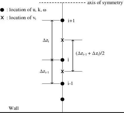
D. Numerical Method

In the numerical method, the non-linear governing equations of the boundary layer for each turbulence models were solved by using a Crank-Nicolson type implicit finite-difference scheme, as shown in Figure 1. In order to achieve better accuracy near the wall, the grid spacing was allowed to increase exponentially. In space 100 and in time 7200 steps per wave cycle were used.

The convergence was achieved through two stages; the first stage of convergence was based on the dimensionless values of u, k and at every time instant during a wave cycle. Second stage of convergence was based on the maximum wall shear stress in a wave cycle. The convergence limit was set to 1x10-6 for both the stages. Full description of the numerical technique, boundary conditions and model parameters are provided in [12-13].

The dimensionless governing equations, i.e. equation of motion (Equation 17), the transport equation of turbulent kinetic energy k (Equation 18) and the transport equation of the specific dissipation rate  (Equation 19) may be expressed in the following form by using a Crank-Nicolson type implicit scheme (omitting the superscript (*));

Equation of motion:



j j



j i j i p p t u u          1 , 1 , 2

1 ₍₁₇₎

                                                1 2 2 2 1 j t E j t E z u Sv R S z z u Sv R S z

Transport equation of turbulent kinetic energy k:

                                                    1 2 2 2 2 , 1 , 2 1 j t k E j t k E j i j i z u v S R S z z k v S R S z t k k                                             1 2 2 2 2 2 1 j t j t z u v S z u v S (18)

   



1



2 *





 k j k j



Transport equation of the specific dissipation rate :

                                                    1 2 2 2 2 , 1 , 2 1 j t E j t E j i j i z v S R S z z v S R S z t        

   



1



2 2 1 2 2 2 2 2 1                                             

 j j

j j t z u z u v

S   





                j z z k S F  

 1

1 2 2 1 2 2 1





                1 2 2 1 1 1 2 j z z k S F  

 (19)

By considering Figure 1, for any variable ;

 

   i i i i i i t E t

E z z z

Sv R S z Sv R S

z  

 _                           1 1 2 / 1 2 2 2  

   1

2 1 1 2 / 1 2                  i i i i i i t E z z z Sv R S   (20)

where, =u,k, the first derivative of any quantity  may be expressed as;

 

       1

1 1 1 1 1 1 1         _                  i i i i i i i i i i i i i i i i z z z z z z z z

z  

     

 (21)

Hereafter, by using the above finite difference scheme all the three governing equations for each turbulence model may be expressed in a general form as follows,

4 1 3 2 1

1 i i i i i i

i A A A

A       (22)

The coefficients 1, 2, 3 and 4 form the elements of a tridiagonal matrix, which may be solved by Gauss elimination method.

E. Experimental Method of Rough Turbulent Boundary Layer

Rough turbulent flow experiments representative of irregular waves were carried out by [19] in an oscillating tunnel using air as the working fluid at Laboratory of Environmental Hydrodynamics Tohoku University Japan. The wind tunnel has a length of 5 m and the height and width of the cross section are 20 cm and 10 cm, respectively. Experimental data has been used for comparisons with model results. The flow measuring unit comprised of a wind tunnel and one component LDV for flow measurement. Velocity measurements were carried out at 21 points in the vertical direction at the center part of the wind tunnel by means of LDV.

The aluminum ball elements of roughness, similar idea used by [26], pasted over the bottom surface of the wind tunnel without spacing along the wind tunnel. The aluminum ball elements were chosen in order to the roughness elements protrude out of the viscous sub-layer. The aluminum balls roughness having a diameter of 10 mm, as depicted in Figure 2. The balls roughness elements also used by [15] in an experimental investigation on wave boundary layers over a bed with large roughness.

Reynolds number is defined using Equation 23, to obtain rough bed turbulent flow was set Re1/3=5.0×10

5 to reach a fully turbulent regime.

3 / 1 2 3 / 1 3 / 1

Re

 U

 ,

3 / 1 3 / 1

2

T



  (23)

where, U1/3: the amplitude of flow velocity based on

parameter of significant wave, T1/3: the significant wave

period, and : the kinematics viscosity.

The spectral density for irregular wave water surface elevation, S_η (f) can be computed using Bretschneider-Mitsuyasu spectral density formulation in the following Equation 24,

 











4



3 / 1 5

3 / 1 3 / 1 2

3 /

1 exp 1.03

257 .

0   

 H T T f T f

f

S_ (24)

where, H1/3, and T1/3 are significant wave height and

period respectively, and f is frequency of component waves. Applying small amplitude wave theory following relationships can be obtained for spectral densities of water surface elevation and free stream velocity, as shown in Equation 25,

 

   

   

f S f

L h f

S f H f

SU U  



 2

2

/ 2 sinh _

 

  

 (25)

where, SU (f) is spectral density for free stream velocity, HU (f) is velocity transfer function, h is water depth, and L and (=2) are wave length and angular frequency of component waves respectively.

Obtained velocity spectrum has been used to generate velocity time variation with the approximation that irregular waves can be resolved as a sum of infinite number of regular wavelets with small amplitudes and random phases, as shown in Equations 26 and 27,

 











i

i i

Ui ft

A t

U cos 2  (26)

 

i

U

Ui S f f

A 2  (27) where, U(t) is instantaneous free stream velocity, AVi are

velocity amplitudes of component waves, fi are

component frequencies, t is time, i are component phases and  are frequency increments between successive wave components.

III.RESULTS AND DISCUSSION A. Mean Velocity Distributions

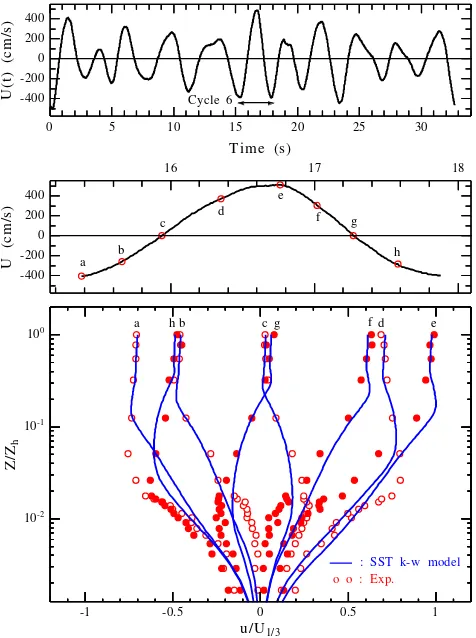
Experiment data of mean velocity profiles in the rough turbulent boundary layer for irregular waves at selected phases were compared with the SST k- model for the second, fifth and sixth cycles presented in Figures 3, 4 and 5, respectively. The second and sixth cycles from the experimental data irregular waves indicated lower and higher of the velocity overshoot while fifth cycle indicated higher period of the velocity overshoot. The solid line showed the turbulence model prediction results by the SST k- model while open and closed rounds showed the experimental data of mean velocity profile.

As depicted in both experimental and the turbulence model display that the velocity overshoot is much influenced by the effect of acceleration and the magnitude of the velocity. The difference of the acceleration between the crest and through phases is significant. The velocity overshoot at phases of D, E and

F the all cycles is higher than that at phases of A, B and H. The mean velocity close to the bottom increases with the increase of the velocity overshoot, corresponding to the increase of the acceleration effect at the crest part of wave motion. The sixth cycle displays that the mean velocity close to the bottom is higher than other cycles.

As seen in these Figures, a good agreement between experimental and the SST k- model has been achieved especially at phases of A, B, E and F for second cycle, and at phases E, F and H for fifth cycle, and at phases B, D, F and H for sixth cycle, when velocityovershooting occurs. The irregularity effectat during acceleration and deceleration phases along a wave cycle where the pressure gradient is very steep in the present irregular wave cases, it seems that the turbulence models have slight difficulties coping with the flow situation. It can be concluded that the SST k- model could predict well the mean velocity distribution for irregular waves especially during acceleration phases for experimental cases considered. The irregularity of the waves affects the dynamic properties of turbulent boundary layer.

After the validation of SST k- model with the experimental data, we determined the roughness effects by using the SST k- model to simulate irregular wave velocity flows with various values of the roughness parameter (am/ks), which increase gradually from am/ks

=5 to am/ks =3122.

Figure 6 shows the predicted results of the mean velocity distribution for Re=5×105 at sixth cycle phases D and E. Roughness tends to decrease the mean velocity in the inner boundary layer. In the outer boundary layer, however, the mean velocity distribution is relatively unaffected by the roughness.

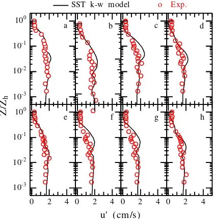
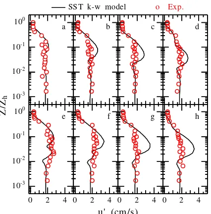
B. Turbulent Intensity and Turbulence Kinetic Energy

Comparison of the turbulent intensity from experimental results for fifth and sixth cycles and the SST k- model prediction at selected phases are given in Figure 7 and 8. The turbulent intensity or the fluctuating velocity in the x-direction u′ from numerical modeling can be estimated using Equation 28 that is a relationship derived from experimental data for steady flow [27]:

k

u'  1.052 (28)

where k is the turbulent kinetic energy obtained in the turbulence model.

Comparisons made on the basis of approximation to calculate the fluctuating velocity by [27] may not be applicable in the whole range of cross-stream dimension in the same manner as the assumption of isotropic turbulence. In the fact that far from the wall, where the flow is practically isotropic, this expression may surely better approximation as compared to the region near the wall where the flow is essentially non-isotropic. The SST

k- model can predict very well the turbulent intensity across the depth at almost all at phases. But, between far and near the wall shows the model slightly overestimates the intensity at phases C, F and G (fifth cycle) and at phases B, C, D, F, G and H (sixth cycle). Moreover, the SST k- model prediction far and near from the bed is generally good. However, the prediction model qualitatively produces very good indication of the pattern of turbulence generation and it mixing.

function of location. Roughness tends to increase the turbulent kinetic energy in the inner boundary layer, in other words, the increase of the roughness causes the increase of the turbulence kinetic energy in the inner boundar layer, while in the outer boundary layer, the turbulent kinetic energy is relatively unaffected for all roughness cases. It is envisaged that the higher roughness yields the higher turbulence kinetic energy that will give a big impact on the sediment transport keeping it in suspension, especially for settling and pick up suspension sediment through turbulence.

C. Bottom Shear Stress

1. Logarithmic Profile and Energy Dissipation Methods Bottom shear stress from experimental data can be estimated by using logarithmic velocity distribution given in Equation 29, as follow,

      

o

z z U

u ln

*

 (29)

where, u is the flow velocity in the boundary layer,  is the von Karman's constant (=0.4), z is the cross-stream distance from theoretical bed level (z=y+Δz) and zo is the

characteristic roughness length denoting the value of z at which the logarithmic velocity profile predicts a velocity of zero. zo can be obtained by applying the Nikuradse's

equivalent roughness in which zo=ks/30; where ksis the

bottom roughness. By plotting µ against ln(z/z0), a

straight line is drawn from log-fitting to measured velocity profile through the experimental data, the value of friction velocity, Ucan be obtained from the slope of this line and bottom shear stress,0 can then be obtained from Equation 30. The obtained values of z and zo as

the above mentioned have a sufficient accuracy for application of logarithmic law in a wide range of velocity profile near bottom region.

* *

U U

o 

  (30)

Roughness elements that have the aluminum balls shape were used to express the bed roughness in this present study. These roughness elements that cause a wake behind each roughness element, and the shear stress is transmitted to the bottom by the pressure drag on the roughness elements. Viscosity becomes irrelevant for determining either the velocity distribution or the overall drag on the surface. Thus, the velocity distribution near a rough bed for steady flow is logarithmic. It may be therefore assumed that log-law can be used to estimate the time variation of bottom shear stress o (t) over rough bed as shown by previous studies i.e. [1]. Hereafter, the bottom shear stress for experimental results can be evaluated with that of turbulence models.

Numerical predictions of turbulence model can be used to predict the bottom shear stress under irregular wave. One of numerical prediction can be using the energy dissipation method. The SST k- model was used to evaluate the bottom shear stress to compare with the experimental data. For a log layer, a local balance between production, P and dissipation of turbulent kinetic energy,  ( = k) can be used to obtain the friction velocity, *

U through the logarithmic velocity profile in Equation 29.

Figure 10 (a) shows the time-variation of bottom shear stress under irregular waves comparison among

experimental results and turbulence models prediction. The SST k- model could predict well the bottom shear stress showing a good agreement with the experimental data along a wave cycle under irregular wave. The SST

k-model has given the underestimate and overestimate values with the experimental data especially at the trough part and the crest part of bottom shear stress. It can be concluded that SST k-model can be used to predict well the bottom shear stress under irregular waves over rough beds.

Figure 10 (b) shows the time histories of the bottom shear stress under irregular wave with various values of the roughness parameter (am/ks), which increase

gradually from am/ks =5 to am/ks =3122. The predicted

results for am/ks =69.38 agree well with the experimental

data along a wave cycle under irregular wave. The increase in roughness increases the magnitude of bottom shear stress, which will influence sediment transport. 2. Comparison with existing calculation approaches

The bottom shear stress for experimental results under irregular waves is examined by the existing calculation approaches. There are two existing estimation approaches of bottom shear stress for irregular wave boundary layers. The maximum bottom shear stress (Method 1) within a basic harmonic wave cycle modified by the phase difference proposed by [14] is given Equation 31,

   

t U t U f

t w

o 

  

2 1

     

  (31)

where o

 

t is the instantaneous bottom shear stress, t is time,  is the angular frequency, U(t) is the time history of free stream velocity,  is phase difference between bottom shear stress and free stream velocity and fwis the

wave friction factor where fw is calculated from Equation

32 as proposed by [28].

   

   

        

0.100

07 . 8 53 . 7 exp

o m w

z a

f (32)

Method 2 is proportional to the square of the instantaneous wave friction velocity, U*(t), which

incorporates the acceleration effect proposed by [11] in Equations 33 and 34. This approach is based on the assumption that the steady flow component is weak (e.g. in a strong undertow, in a surf zone, etc.).

     

   

 

   

t t U t

U f

t

U* w/2 cos sin

(33)

 

t U

   

t U t

o  * *

  (34)

The phase difference for calculating in Method 1 and Method 2 can be obtained from significant wave quantities, instead of calculating for individual waves, as given in Equation 37.

563 . 0

357 . 0 153

. 0

127 . 0 1

00279 . 0 1 4 . 42

C C C

 

 

 (degree) (35)

o m w

z a f C

2 1



 for rough bed condition (36)

T T 



 4

2

Friction coefficient used in Method 2 is calculated from Equation 38 as proposed by [29], as follows:

                 3 , 6 5 , 5 exp 2 , 0 s m w k a

f (38)

3. A new calculation approaches

The first new calculation approach of bottom shear stress under irregular waves (Method 3) is based on incorporating velocity and acceleration terms all at once that is given through the instantaneous friction velocity,

U*(t) as proposed by [12-13] in Equation 39. Both velocity and acceleration terms are adopted from the calculation method proposed by [11]. The phase difference was determined from an empirical formula for practical purposes. The instantaneous friction velocity can be expressed as:

 

 

                 t t U a t U f t

U _w c

  

2 /

* ₍₃₉₎

where, fw: the wave friction coefficient as given in

Equation 32 can be used for evaluating in Equation 36.



: the phase difference between free stream velocity and bottom shear stress. Phase difference equation given in Equation 35 is used for calculating in Method 3.

The value of acceleration coefficient, ac is determined

empirically from both experimental and Shear Stress Transport (SST) k- numerical model results of bottom shear stress using following relationship as shown in Equation (40).       t t U f t U f t U t a w w c               2 / 2 / * (40)

Here, the value of acceleration coefficient, ac = 0.485,

is obtained from average value of the time variation of acceleration coefficient ac(t) calculated from

experimental result as well as the SST k- numerical model results of bottom shear stress, and is using to expressed irregularity form effect under irregular wave.

The instantaneous bottom shear stress o(t) can be

calculated proportional to the square of the proposed instantaneous friction velocity, as shown in Equation 41.

 

t U

   

t U t

o

* *



  (41)

The second new calculation approach of bottom shear stress under irregular waves (Method 4) is derived from the time–variation of bottom shear stress for an arbitrary variation of U(t) in Equation 42 as proposed by [30].

 

t f_wU

   

t Ut

o

2



  (42)

The value of wave friction coefficient is calculated from Equation 43.

16 . 0 041 . 0   _e w R

f (43)

Investigation of laminar bottom boundary layer under irregular waves as proposed by [31] is constructed the time–variation of bottom shear stress in Equation 44.

 

 

0.16

   

0.68

041 . 0

2 Ut U t

t

o 



  (44)

This estimation of bottom shear stress is obtained a good agreement with experiment results of laminar bottom boundary layer under irregular waves. However, this estimation cannot be used to condition for turbulence

flow was analyzed in this research. The bottom shear stress for laminar flow is resulted too small according to the value of Reynold number far smaller than the turbulence flow.

The hydrodynamics conditions were observed subsequently and interpreted using bottom shear stress, phase difference and friction factor for rough bed. The wave friction coefficient for rough turbulent is defined as follows [32],                06 . 2 1 0101 . 0 exp R R f e w with

 

 

0.16

   

0.68

184 . 0

039 .

0 U t U t

k a

t a a

s m

o  

 _     

 (46)

 

                 t t U a t U t U c a ) (  

 ₍₄₇₎

where am/ks is the roughness parameter, ks can be

obtained by applying the Nikuradse's equivalent roughness in which ks= 2.5 d50,  is frequency angular, Ua(t) is the time history of free stream velocity as

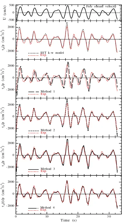
proposed by [12-13] without the wave friction effect. Comparison among the experimental data, SST k- turbulence model and calculation approaches for bottom shear stress estimation under irregular waves are given in Figure 11. Method 4 could predict well the bottom shear stress showing the best agreement with the experimental results along a wave cycle under irregular wave than other methods and SST k- turbulence model. SST k- turbulence model gave overestimated value at both though and crest parts of bottom shear stress from experimental results. While Method 1, Method 2 and Method 3 have given underestimated and overestimated values of the bottom shear stress with the experimental data especially value at trough part and crest part, respectively. While, SST k- model and Method 1 was not so much in a good agreement with the experimental results along a wave cycle under irregular wave due to was not exclude the velocity and acceleration effect in the calculation of the bottom shear stress.

Further, the calculation approach performance of bottom shear stress can be evaluated by the Root-Mean-Square Error (RMSE), as follows:

 







 









   N 1 i 2 exp o cal

o t / t /

N 1

RSME     (48)

where, (o(t)/)cal is the bottom shear stress from

calculation approaches, (o(t)/)exp is the bottom shear stress from experimental results, N is the total number of data and i is index. The calculation approach agreement with experimental data when the RMSE is zero. The summary of the calculation approach performance of bottom shear stress is in perfect performance for bottom shear stress can be seen in Table 2.

IV.CONCLUSION

The predictions of turbulent boundary layer for irregular waves over rough beds have been investigated by the SST k- turbulence model validated by the available experimental data. The SST k- model could predict well the mean velocity, turbulent intensity and kinetic energy and bottom shear stress for irregular waves. The effect of roughness on the turbulent boundary layers under irregular waves were also studied using the SST k- turbulence model. Roughness tends to decrease the mean velocity and to increase the turbulent kinetic energy in the inner boundary layer, whereas in the outer boundary layer, while the roughness alters the turbulent kinetic energy and the mean velocity distribution is relatively unaffected. Moreover, the higher roughness elements also increase the magnitude of the bottom shear stress along wave cycle.

The second new approach of estimating bottom shear stress under irregular waves (Method 4) has shown a

good agreement with the experimental data and the SST

k- numerical model. Therefore, method 4 may be considered as a reliable calculation method of bottom shear stress under irregular waves.

ACKNOWLEDGEMENT

The authors are grateful for the support provided by Sepuluh November Institute of Technology and DP2M-DIKTI. This research was partially supported by Grant of Hibah Bersaing DP2M DIKTI 2011 (No: 044/SP2H/ PL/Dit.Litabmas/IV/2011) and by Grant of PUM ITS 2011 (No. 0750.185/I2.7/PM/2011, May 02, 2011). This research is also part of Doctoral study of first author in Institut Teknologi Sepuluh Nopember (ITS) Surabaya which is supported by Ministry of National Education

Hasanuddin University Engineering Faculty

Development Project JBIC Loan No.IP-541 through Fellowship Doctoral Degree Program in-Country. The authors would like to gratefully appreciate these financial supports.

Δzi

(Δzi-1 + Δzi)/2

Δzi-1

i-1

i

i+1

x

x

axis of symmetry

Wall

: location of u, k, ω

: location of vt

x

Figure 1. Finite difference scheme

D=10mm Hr = 10 mm

z = 0 zo u

∆z

z

y = 0

y _u

0 5 10 15 20 25 30 -400

-200 0 200 400

U

(t

)

(c

m

/s

)

Cycle 2

3 4 5

Tim e (s)

-400 -200 0 200 400

U

(c

m

/s

)

a b

c

d e f

g h

a hb gcfde

: SST k-w model o o : Exp.

-1 -0.5 0 0.5 1

u/U1/3

10-2

10-1

100

Z

/Z

h

Figure 3. Mean velocity profile for the second cycle of irregular waves

0 5 10 15 20 25 30

-400 -200 0 200 400

U

(t

)

(c

m

/s

) Cycle 5

11 12 13 14 15

Time (s)

-400 -200 0 200 400

U

(c

m

/s

)

a b

c

d e f

g

h

-1 -0.5 0 0.5 1

u/U1/3

10-2

10-1

100

Z

/Z

h

a h b gc dfe

: SST k-w model o o : Exp.

Figure 4. Mean velocity profile for the fifth cycle of irregular waves

0 5 10 15 20 25 30

-400 -200 0 200 400

U

(t

)

(c

m

/s

)

Cycle 6

16 17 18

Tim e (s)

-400 -200 0 200 400

U

(c

m

/s

)

a b

c d

e

f _g

h

-1 -0.5 0 0.5 1

u/U1/3 10-2

10-1 100

Z

/Z

h

a hb cg fd e

: SST k-w model o o : Exp.

10- 1 ₁₀0

u/U1/3

10-4

10-3

10-2

10-1

100

Z

/Z

h

Phase E

10-4

10-3

10-2

10-1

100

Z

/Z

h

Model am/ks=5

Model am/ks=69.38

Model am/ks=3122

Phase D

Figure 6. Effect of roughness on the mean velocity distributions for the sixth cycle of irregular waves

10-3

10-2

10-1

100

SST k-w model o Exp.

a

Z

/Z

h

b c d

0 2 4

10-3

10-2

10-1

100

e

0 2 4

f

u' (cm /s)

0 2 4

g

0 2 4

h

Figure 8. Turbulent intensity comparison of the SST k-ω model prediction and experimental data for the sixth cycle of irregular waves

0 2 4 6

k 10-3

10-2

10-1

100

Z

/Z

h

Phase E 10-3

10-2

10-1

100

Z

/Z

h

Model am/ks=5

Model am/ks=69.38

Model am/ks=3122

Phase D

Figure9. Effect of roughness on the turbulence kinetic energy distributions for the sixth cycle of irregular waves

0 10 20 30

Tim e (s)

-2000 0 2000

o

(t

)/



(c

m

2 /s 2 )

Model am/ks=5

Model am/ks=69.38

Model am/ks=3122

-2000 0 2000

o

(t

)/



(c

m

2 /s 2 )

SST k-w Model Exp. -500

0 500

U

(c

m

/s

)

Figure 10. (a). Bottom shear stress comparison among experimental results and turbulence models prediction , (b).

Effect of roughness on the bottom shear stress

10-3

10-2

10-1

100

SST k-w model o Exp.

Z

/Z

h

a b c d

0 2 4

10-3

10-2

10-1

100

e

0 2 4

f

u' (cm /s)

0 2 4

g

0 2 4

-500 0 500

U

(c

m

/s

) Free stream velocity

-2000 0 2000

o

/



(c

m

2/s 2)

SST k-w model

Exp.

-2000 0 2000

o

/



(c

m

2/s 2)

Method 1

Exp.

-2000 0 2000

o

/



(c

m

2/s 2)

Method 2

Exp.

-2000 0 2000

o

/



(c

m

2/s 2)

Method 3

Exp.

0 10 20 30

Time (s)

-2000 0 2000

o

(t

)/



(c

m

2/s 2)

Method 4

Exp.

Figure 11. Comparison for bottom shear stress estimation

TABLE 1. INPUT WAVE PARAMETERS

Exp. U1/3(cm/s) T1/3 (s) v

(cm2/s) Re am/ks

1 392 3.0 0.148 5.0 ×105 _69.38

TABLE 2.

THE SUMMARY OF CALCULATION APPROACH PERFORMANCE FOR BOTTOM SHEAR STRESS

Exp.

The Root-Mean-Square Error (RMSE)

Method 1 Method 2 Method 3 Method 4

Case 1 3.79 7.68 1.60 1.25

REFERENCES

[1] I. G. Jonsson and N. A. Carlsen, “Experimental and theoretical investigations in an oscillatory turbulent boundary layer,”Journal

of Hydraulic Research, vol.14, no.1, pp. 45-60, 1976.

[2] M. Hino, M. Kashiwayanag, A. Nakayama, and T. Nara,

“Experiments on the turbulence statistics and the structure of a reciprocating oscillatory flow,”Journal Fluid Mechanic, vol.131, pp. 363-400, 1983.

[3] J. F. A. Sleath, “Turbulent oscillatory flow over rough beds,”

Journal of Fluid Mechanics, vol.182, pp. 369-409, 1987.

[4] B.L. Jensen, B.M. Sumer, and J. Fredsøe,” Turbulent oscillatory boundary layers at high Reynolds numbers,” Journal Fluid Mech., vol.206, pp. 265-297, 1989.

[5] Suntoyo and H. Tanaka, “Experimental studi on a smooth bed boundary layer flows under solitary wave,” Tohoku Journal of

Natural Disaster Science, vol.44, pp. 197-202, 2008.

[6] J. Fredsøe, B. M. Sumer, A. Kozakiewiecz, L. H. C. Chua, and R.

Diegaard, ”Effect of externally generated turbulence on wave boundary layer,”Coastal Engineering, vol.49, pp. 155-183, 2003. [7] M.A. Samad and H. Tanaka, “Numerical investigations on irregular wave bottom boundary layer under laminar motion,”

Coastal Engineering and Marine Developments, (Ed. Brebbia,

C.A. and Anagnostopoulos, P.), WIT Press, pp. 193-202, 1999. [8] M.A. Samad and H. Tanaka, “Estimating instantaneous turbulent

bottom shear stress under irregular wave,” Journal of

Hydroscience and Hydraulic Engineering, vol.17, no.2, pp.

107-126, 1999.

[9] A.G. Davies, “A Numerical model of the wave boundary layer,”

Continental Shelf Research, vol.6. no.6, pp. 715-739, 1986.

[10] A. Sana, H. Tanaka and T. Suzuki, “Experimental and numerical study of irregular wave boundary layers on a rough bottom,”

Coastal Engineering, vol. 34, pp. 521-528, 2004.

[11] P. Nielsen, “Shear stress and sediment transport calculations for swash zone modeling,”Coastal Engineering, vol. 45, pp. 53–60, 2002.

[12] Suntoyo, H. Tanaka and A. Sana, “Characteristics of turbulent boundary layers over a rough bed under saw-tooth waves and its application to sediment transport,”Coastal Engineering, vol. 55, no. 12, pp. 1102-1112, 2008.

[13] Suntoyo and H. Tanaka, “Effect of bed roughness on turbulent boundary layer and net sediment transport under asymmetric waves,”Coastal Engineering, vol. 56, no. 9, 2009, pp. 960-969. [14] H. Tanaka and M.A. Samad , “Prediction of instantaneous bottom

shear stress for turbulent plane bed condition under irregular wave,”Journal of Hydraulic Research Elsevier, vol.44, no.1, pp. 94-106, 2006.

[15] M. Dixen, F. Hatipoglu, B.M.Sumer, and J. Fredsøe, “Wave boundary layer over a stone-covered bed,”Coastal Engineering, vol. 55, pp. 1-20, 2008.

[16] Suntoyo and H. Tanaka,“Numerical Modeling of boundary layer flows for a solitary wave,” Journal of Hydro-environment

[17] H. Tanaka, B. Winarta, Suntoyo and H. Yamaji, “Validation of a new generation system for bottom boundary layer beneath solitary wave,”Coastal Engineering, vol. 59, pp.46-56, 2011. [18] F. R. Menter, “Two-equation eddy-viscosity turbulence models

for engineering applications,” AIAA Journal, vol.32, no.8, pp.1598-1605, 1994.

[19] H. Tanaka, T. Suzuki, Suntoyo and H. Yamaji, “Time-variation

of bottom shear stress under irregular waves over rough bed,”

Journal of Hydroscience and Hydraulic Engineering, vol.25,

no.2, pp. 217-225, 2002.

[20] T. Rachman, and Suntoyo, “A new method for modeling bottom

shear stress under irregular waves,” IPTEK The Journal for

Technology and Science, vol.22, no.2, May 2011.

[21] A. Sana and E. B. Shuy, “Two-equation turbulence models for smooth oscillatory boundary layers,”Journal of Waterway, Port,

Coastal and Ocean Engineering, pp. 38-45, January-February

2002.

[22] ANSYS, “The CFX approach to turbulence modeling: Accurate

and effective turbulent flow simulations,” CFX Technical Brief, PDF0072 07/03, Available: http://www.ansys.com/cfx.

[23] Suntoyo, “Study on turbulent bottom boundary layer under non

-linier waves and its application to sediment transport,“ Ph.D. Dissertation, Tohoku University, Japan, 2006.

[24] D. C. Wilcox, “Reassessment of the scale-determining equation

for advanced turbulent models,” AIAA Journals, vol.26, no.11,

pp. 1299-1310, 1988.

[25] P. G. Saffman, “Dependence on Reynolds number of high-order

moments of velocity derivatives in isotropic turbulence,”Phys.

Fluids 13, pp. 2192-2193, 1970.

[26] P. Justesen, “Turbulent wave boundary layer,” Series Paper

no. 43, ISVA, Technical University of Denmark, 1988.