Pattern Recognition Introduction, Features, Classifiers and Principles pdf pdf

(1)

(2)

Jürgen Beyerer, Matthias Richter, Matthias Nagel

Pattern Recognition

(3)

Also of Interest

Dynamic Fuzzy Machine Learning L. Li, L. Zhang, Z. Zhang, 2018

ISBN 978-3-11-051870-2, e-ISBN 978-3-11-052065-1,

e-ISBN (EPUB) 978-3-11-051875-7, Set-ISBN 978-3-11-052066-8

Lie Group Machine Learning F. Li, L. Zhang, Z. Zhang, 2019

ISBN 978-3-11-050068-4, e-ISBN 978-3-11-049950-6,

Complex Behavior in Evolutionary Robotics L. König, 2015

ISBN 978-3-11-040854-6, e-ISBN 978-3-11-040855-3,

(4)

Pattern Recognition on Oriented Matroids A. O. Matveev, 2017

ISBN 978-3-11-053071-1, e-ISBN 978-3-11-048106-8,

Graphs for Pattern Recognition D. Gainanov, 2016

ISBN 978-3-11-048013-9, e-ISBN 978-3-11-052065-1,

(5)

(6)

Authors

Institute of Anthropomatics and Robotics, Chair IES Karlsruhe Institute of Technology Adenauerring 4

76131 Karlsruhe Matthias Richter

Institute of Anthropomatics and Robotics, Chair IES Karlsruhe Institute of Technology Adenauerring 4

76131 Karlsruhe

matthias.richter@kit.edu Matthias Nagel

Institute of Theoretical Informatics, Cryptography and IT Security Karlsruhe Institute of Technology Am Fasanengarten 5

A CIP catalog record for this book has been applied for at the Library of Congress.

Bibliographic information published by the Deutsche Nationalbibliothek

The Deutsche Nationalbibliothek lists this publication in the Deutsche Nationalbibliografie; detailed bibliographic data are available on the Internet at http://dnb.dnb.de.

(7)

Preface

PATTERN RECOGNITION ⊂ MACHINE LEARNING ⊂ ARTIFICIAL INTELLIGENCE: This relation could give

the impression that pattern recognition is only a tiny, very specialized topic. That, however, is misleading. Pattern recognition is a very important field of machine learning and artificial intelligence with its own rich structure and many interesting principles and challenges. For humans, and also for animals, their natural abilities to recognize patterns are essential for navigating the physical world which they perceive with their naturally given senses. Pattern recognition here performs an important abstraction from sensory signals to categories: on th most basic level, it enables the classification of objects into “Eatable” or “Not eatable” or, e.g., into “Friend” or “Foe.” These categories (or, synonymously, classes) do not always have a tangible character. Examples of non-material classes are, e.g., “secure situation” or “dangerous situation.” Such classes may even shift depending on the context, for example, when deciding whether an action is socially acceptable or not. Therefore, everybody is very much acquainted, at least at an intuitive level, with what pattern recognition means to our daily life. This fact is surely one reason why pattern recognition as a technical subdiscipline is a source of so much inspiration for scientists and engineers. In order to implement pattern recognition capabilities in technical systems, it is necessary to formalize it in such a way, that the designer of a pattern recognition system can systematically engineer the algorithms and devices necessary for a technical realization. This textbook summarizes a lecture course about pattern recognition that one of the authors (Jürgen Beyerer) has been giving for students of technical and natural sciences at the Karlsruhe Institute of Technology (KIT) since 2005. The aim of this book is to introduce the essential principles, concepts and challenges of pattern recognition in a comprehensive and illuminating presentation. We will try to explain all aspects of pattern recognition in a well understandable, self-contained fashion. Facts are explained with a mixture of a sufficiently deep mathematical treatment, but without going into the very last technical details of a mathematical proof. The given explanations will aid readers to understand the essential ideas and to comprehend their interrelations. Above all, readers will gain the big picture that underlies all of pattern recognition.

The authors would like to thank their peers and colleagues for their support:

Special thanks are owed to Dr. Ioana Gheța who was very engaged during the early phases of the lecture “Pattern Recognition” at the KIT. She prepared most of the many slides and accompanied the course along many lecture periods.

Thanks as well to Dr. Martin Grafmüller and to Dr. Miro Taphanel for supporting the lecture Pattern Recognition with great dedication.

Moreover, many thanks to to Prof. Michael Heizmann and Prof. Fernando Puente León for inspiring discussions, which have positively influenced to the evolution of the lecture.

Thanks to Christian Hermann and Lars Sommer for providing additional figures and examples of deep learning. Our gratitude also to our friends and colleagues Alexey Pak, Ankush Meshram, Chengchao Qu, Christian Hermann, Ding Luo, Julius Pfrommer, Julius Krause, Johannes Meyer, Lars Sommer, Mahsa Mohammadikaji, Mathias Anneken, Mathias Ziearth, Miro Taphanel, Patrick Philipp, and Zheng Li for providing valuable input and corrections for the preparation of this manuscript.

Lastly, we thank De Gruyter for their support and collaboration in this project.

Karlsruhe, Summer 2017

(8)

(9)

List of Tables

Table 1 Capabilities of humans and machines in relation to pattern recognition

Table 2.1 Taxonomy of scales of measurement

Table 2.2 Topology of the letters of the German alphabet

Table 7.1 Character sequences generated by Markov models of different order

(14)

List of Figures

Fig. 1 Examples of artificial and natural objects Fig. 2 Industrial bulk material sorting system

Fig. 1.1 Transformation of the domain into the feature space M Fig. 1.2 Processing pipeline of a pattern recognition system Fig. 1.3 Abstract steps in pattern recognition

Fig. 1.4 Design phases of a pattern recognition system

Fig. 1.5 Rule of thumb to partition the dataset into training, validation and test sets

Fig. 2.1 Iris flower dataset

Fig. 2.2 Full projection and slice projection techniques Fig. 2.3 Construction of two-dimensional slices

Fig. 2.4 Feature transformation for dimensionality reduction Fig. 2.5 Unit circles for different Minkowski norms

Fig. 2.6 Kullback–Leibler divergence between two Bernoulli distributions Fig. 2.7 KL divergence of Gaussian distributions with equal variance Fig. 2.8 KL divergence of Gaussian distributions with unequal variances Fig. 2.9 Pairs of rectangle-like densities

Fig. 2.10 Combustion engine, microscopic image of bore texture and texture model Fig. 2.11 Systematic variations in optical character recognition

Fig. 2.12 Tangential distance measure

Fig. 2.13 Linear approximation of the variation in Figure 2.11 Fig. 2.14 Chromaticity normalization

Fig. 2.15 Normalization of lighting conditions

Fig. 2.16 Images of the surface of agglomerated cork Fig. 2.17 Adjustment of geometric distortions

Fig. 2.18 Adjustment of temporal distortions

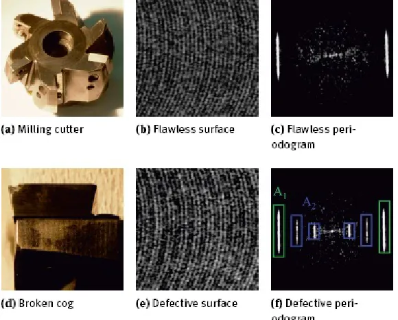
Fig. 2.19 Different bounding boxes around an object Fig. 2.20 The convex hull around a concave object Fig. 2.21 Degree of compactness (form factor) Fig. 2.22 Classification of faulty milling cutters

Fig. 2.23 Synthetic honing textures using an AR model

Fig. 2.24 Physical formation process and parametric model of a honing texture Fig. 2.25 Synthetic honing texture using a physically motivated model

Fig. 2.26 Impact of object variation and variation of patterns on the features Fig. 2.27 Synthesis of a two-dimensional contour

Fig. 2.28 Principal component analysis, first step Fig. 2.29 Principal component analysis, second step Fig. 2.30 Principal component analysis, general case

Fig. 2.31 The variance of the dataset is encoded in principal components Fig. 2.32 Mean face of the YALE faces dataset

Fig. 2.33 First 20 eigenfaces of the YALE faces dataset

Fig. 2.34 First 20 eigenvalues corresponding to the eigenfaces in Figure 2.33 Fig. 2.35 Wireframe model of an airplane

Fig. 2.36 Concept of kernelized PCA

(15)

Fig. 2.42 First ten Fisher faces of the YALE faces dataset Fig. 2.43 Workflow of feature selection

Fig. 2.44 Underlying idea of bag of visual words Fig. 2.45 Example of a visual vocabulary Fig. 2.46 Example of a bag of words descriptor Fig. 2.47 Bag of words for bulk material sorting

Fig. 2.48 Structure of the bag of words approach in Richter et al. [2016]

Fig. 3.1 Example of a random distribution of mixed discrete and continuous quantities Fig. 3.2 The decision space K

Fig. 3.3 Workflow of the MAP classifier

Fig. 3.4 3-dimensional probability simplex in barycentric coordinates

Fig. 3.5 Connection between the likelihood ratio and the optimal decision region Fig. 3.6 Decision of an MAP classifier in relation to the a posteriori probabilities Fig. 3.7 Underlying densities in the reference example for classification

Fig. 3.8 Optimal decision regions Fig. 3.9 Risk of the Minimax classifier

Fig. 3.10 Decision boundary with uneven priors

Fig. 3.11 Decision regions of a generic Gaussian classifier

Fig. 3.12 Decision regions of a generic two-class Gaussian classifier

Fig. 3.13 Decision regions of a Gaussian classifier with the reference example

Fig. 4.1 Comparison of estimators

Fig. 4.2 Sequence of Bayesian a posteriori densities

Fig. 5.1 The triangle of inference

Fig. 5.2 Comparison of Parzen window and k-nearest neighbor density estimation Fig. 5.3 Decision regions of a Parzen window classifier

Fig. 5.4 Parzen window density estimation (m∈ R) Fig. 5.5 _{Parzen window density estimation (}_m∈ R2) Fig. 5.6 k-nearest neighbor density estimation

Fig. 5.7 Example Voronoi tessellation of a two-dimensional feature space Fig. 5.8 Dependence of the nearest neighbor classifier on the metric Fig. 5.9 k-nearest neighbor classifier

Fig. 5.10 Decision regions of a nearest neighbor classifier Fig. 5.11 Decision regions of a 3-nearest neighbor classifier Fig. 5.12 Decision regions of a 5-nearest neighbor classifier

Fig. 5.13 Asymptotic error bounds of the nearest neighbor classifier

Fig. 6.1 Increasing dimension vs. overlapping densities

Fig. 6.2 Dependence of error rate on the dimension of the feature space in Beyerer [1994] Fig. 6.3 Density of a sample for feature spaces of increasing dimensionality

Fig. 6.4 Examples of feature dimension d and parameter dimension q

Fig. 6.5 Trade-off between generalization and training error Fig. 6.6 Overfitting in a regression scenario

Fig. 7.1 Techniques for extending linear discriminants to more than two classes Fig. 7.2 Nonlinear separation by augmentation of the feature space.

Fig. 7.3 Decision regions of a linear regression classifier Fig. 7.4 Four steps of the perceptron algorithm

Fig. 7.5 Feed-forward neural network with one hidden layer Fig. 7.6 Decision regions of a feed-forward neural network

(16)

Fig. 7.9 Comparison of ReLU and sigmoid activation functions Fig. 7.10 A single convolution block in a convolutional neural network Fig. 7.11 High level structure of a convolutional neural network.

Fig. 7.12 Types of features captured in convolution blocks of a convolutional neural network Fig. 7.13 Detection and classification of vehicles in aerial images with CNNs

Fig. 7.14 Structure of the CNN used in Herrmann et al. [2016] Fig. 7.15 Classification with maximum margin

Fig. 7.16 Decision regions of a hard margin SVM

Fig. 7.17 Geometric interpretation of the slack variables ξ_i, i = 1, . . . , N. Fig. 7.18 Decision regions of a soft margin SVM

Fig. 7.19 Decision boundaries of hard margin and soft margin SVMs Fig. 7.20 Toy example of a matched filter

Fig. 7.21 Discrete first order Markov model with three states ω_i. Fig. 7.22 Discrete first order hidden Markov model

Fig. 8.1 Decision tree to classify fruit

Fig. 8.2 Binarized version of the decision tree in Figure 8.1 Fig. 8.3 Qualitative comparison of impurity measures Fig. 8.4 Decision regions of a decision tree

Fig. 8.5 Structure of the decision tree of Figure 8.4

Fig. 8.6 Impact of the features used in decision tree learning Fig. 8.7 A decision tree that does not generalize well.

Fig. 8.8 Decision regions of a random forest Fig. 8.9 Strict string matching

Fig. 8.10 Approximate string matching

Fig. 8.11 String matching with wildcard symbol *

Fig. 8.12 Bottom up and top down parsing of a sequence

Fig. 9.1 Relation of the world model P(m,ω) and training and test sets D and D. Fig. 9.2 Sketch of different class assignments under different model families

Fig. 9.3 Expected test error, empirical training error, and VC confidence vs. VC dimension Fig. 9.4 Classification error probability

Fig. 9.5 Classification outcomes in a 2-class scenario Fig. 9.6 Performance indicators for a binary classifier Fig. 9.7 Example of ROC curves

Fig. 9.8 Converting a multi-class confusion matrix to binary confusion matrices Fig. 9.9 Five-fold cross-validation

Fig. 9.10 Schematic example of AdaBoost training.

Fig. 9.11 AdaBoost classifier obtained by training in Figure 9.10 Fig. 9.12 Reasons to refuse to classify an object

Fig. 9.13 Classifier with rejection option

(17)

Notation

General identifiers

a, ..., z Scalar, function mapping to a scalar, or a realization of a random variable

a, ..., z Random variable (scalar)

a, ..., z Vector, function mapping to a vector, or realization of a vectorial random variable

a, ..., z Random variable (vectorial)

â, ..., Realized estimator of denoted variable

â, ..., Estimator of denoted variable as random variable itself

A, ..., Z Matrix

p(m) Probability density function for random variable m evaluated at m

P(ω) Probability mass function for (discrete) random variable ω evaluated at ω

(18)

( ) Power set, i.e., the set of all subsets of Set of real numbers

Set of all samples, S = D ⊎ T ⊎ V

T Set of test samples

V Set of validation samples

U Unit matrix, i.e., the matrix all of whose entries are 1

θ Parameter vector

⇝ Leads to (not necessarily in a strict mathematical sense)

⊎ Disjoint union of sets, i.e., C = A ⊎ B ⇔ C = A ∪ B and A ∩ B = 0.

N(μ, Σ) Multivariate normal/Gaussian distribution with expectation μ and covariance matrix Σ tr A Trace of the matrix A

Var{⋅} Variance

Abbreviations

iff if and only if

i.i.d. independent and identically distributed N.B. “Nota bene” (latin: note well, take note)

(19)

Introduction

The overall goal of pattern recognition is to develop systems that can distinguish and classify objects. The range of possible objects is vast. Objects can be physical things existing in the real world, like banknotes, as well as non-material entities, e.g., e-mails, or abstract concepts such as actions or situations. The objects can be of natural origin or artificially created. Examples of objects in pattern recognition tasks are shown in Figure 1.

On the basis of recorded patterns, the task is to classify the objects into previously assigned classes by defining and extracting suitable features. The type as well as the number of classes is given by the classification task. For example, banknotes (see Figure 1b) could be classified according to their monetary value or the goal could be to discriminate between real and counterfeited banknotes. For now, we will refrain from defining what we mean by the terms pattern, feature, and class. Instead, we will rely on an intuitive understanding of these concepts. A precise definition will be given in the next chapter.

From this short description, the fundamental elements of a pattern recognition task and the challenges to be encountered at each step can be identified even without a precise definition of the concepts pattern, feature, and class:

Pattern acquisition, Sensing, Measuring In the first step, suitable properties of the objects to be classified have to be gathered and put into computable representations. Although pattern might suggest that this (necessary) step is part of the actual pattern recognition task, it is not. However, this process has to be considered so far as to provide an awareness of any possible complications it may cause in the subsequent steps. Measurements of any kind are usually affected by random noise and other disturbances that, depending on the application, can not be mitigated by methods of metrology alone: for example, changes of lighting conditions in uncontrolled and uncontrollable environments. A pattern recognition system has to be designed so that it is capable of solving the classification task regardless of such factors.

Feature definition, Feature acquisition Suitable features have to be selected based on the available patterns and methods for extracting these features from the patterns have to be defined. The general aim is to find the smallest set of the most informative and discriminative features. A feature is discriminative if it varies little with objects within a single class, but varies significantly with objects from different classes.

(20)

Fig. 1. Examples of artificial and natural objects.

These lecture notes on pattern recognition are mainly concerned with the last two issues. The complete process of designing a pattern recognition system will be covered in its entirety and the underlying mathematical background of the required building blocks will be given in depth.

Pattern recognition systems are generally parts of larger systems, in which pattern recognition is used to derive decisions from the result of the classification. Industrial sorting systems are typical of this (see Figure 2). Here, products are processed differently depending on their class memberships.

(21)

Fig. 2. Industrial bulk material sorting system.

Table 1. Capabilities of humans and machines in relation to pattern recognition.

Association & cognition Combinatorics & precision

Human very good poor

(22)

1 Fundamentals and definitions

The aim of this chapter is to describe the general structure of a pattern recognition system and properly define the fundamental terms and concepts that were partially used in the Introduction already. A description of the generic process of designing a pattern recognizer will be given and the challenges at each step will be stated more precisely.

1.1 Goals of pattern recognition

The purpose of pattern recognition is to assign classes to objects according to some similarity properties. Before delving deeper, we must first define what is meant by class and object. For this, two mathematical concepts are needed: equivalence relations and partitions.

Definition 1.1 (Equivalence relation). Let Ω be a set of elements with some relation ∼. Suppose further that o, o₁, o₂, o₃∈Ω are arbitrary. The relation ∼ is said to be an equivalence relation if it different approach to classifying every element of a set is given by partitioning the set:

Definition 1.2 (Partition, Class). Let Ω be a set and ω₁, ω₂, ω₃, . . . ⊆Ω be a system of subsets. This system of subsets is called a partition of Ω if the following conditions are met:

1. ω_i∩ ∩ ω_j= 0 for all i ≠ j, i.e., the subsets are pairwise disjoint, and 2. ω_i= Ω, i.e., the system is exhaustive.

Every subset ω is called a class (of the partition).

It is easy to see that equivalence relations and partitions describe synonymous concepts: every equivalence relation induces a partition, and every partition induces an equivalence relation.

(23)

into classes ω₁, ω₂, ω₃, . . . ⊆Ω. A suitable mapping associates every object o_it to a feature vector

m_i ∈ M inside the feature space M. The goal is now to find rules that partition M along decision

boundaries so that the classes of M match the classes of the domain. Hence, the rule for classifying an object o is

Fig. 1.1. Transformation of the domain Ω into the feature space M.

This means that the estimated class ̂ω(o) of object o is set to the class ω_ii if the feature vector m

(o) falls inside the region R_i. For this reason, the R_i are also called decision regions. The concept of a

classifier can now be stated more precisely:

Definition 1.3 (Classifier). A classifier is a collection of rules that state how to evaluate feature vectors in order to sort objects into classes. Equivalently, a classifier is a system of decision boundaries in the feature space.

Readers experienced in machine learning will find these concepts very familiar. In fact, machine learning and pattern recognition are closely intertwined: pattern recognition is (mostly) supervised learning, as the classes are known in advance. This topic will be picked up again later in this chapter.

1.2 Structure of a pattern recognition system

(24)

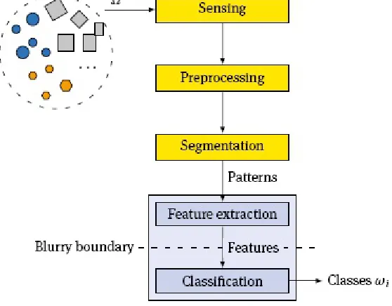
Fig. 1.2. Processing pipeline of a pattern recognition system.

Figure 1.2 shows the processing pipeline of a pattern recognition system. In the first steps, the relevant properties of the objects from Ω must be put into a machine readable interpretation. These first steps (yellow boxes in Figure 1.2) are usually performed by methods of sensor engineering, signal processing, or metrology, and are not directly part of the pattern recognition system. The result of these operations is the pattern of the object under inspection.

Definition 1.4 (Pattern). A pattern is the collection of the observed or measured properties of a single object.

The most prominent pattern is the image, but patterns can also be (text) documents, audio recordings, seismograms, or indeed any other signal or data. The pattern of an object is the input to the actual pattern recognition, which is itself composed of two major steps (gray boxes in Figure 1.2): previously defined features are extracted from the pattern and the resulting feature vector is passed to the classifier, which then outputs an equivalence class according to Equation (1.2).

Definition 1.5 (Feature). A feature is an obtainable, characteristic property, which will be the basis for distinguishing between patterns and therefore also between the underlying classes.

A feature is any quality or quantity that can be derived from the pattern, for example, the area of a region in an image, the count of occurrences of a key word within a text, or the position of a peak in an audio signal.

As an example, consider the task of classifying cubical objects as either “small cube” or “big cube” with the aid of a camera system. The pattern of an object is the camera image, i.e., the pixel representation of the image. By using suitable image processing algorithms, the pixels that belong to the cube can be separated from the pixels that show the background and the length of the edge of the cube can be determined. Here, “edge length” is the feature that is used to classify the object into the classes “big” or “small.”

(25)

conjunction with a powerful classifier, or of combining elaborate features with a simple classifier.

1.3 Abstract view of pattern recognition

From an abstract point of view, pattern recognition is mapping the set of objects Ω to be classified to the equivalence classes ω∈Ω/ ∼, i.e., Ω→Ω/ ∼ or o↦ω. In some cases, this view is sufficient for treating the pattern recognition task. For example, if the objects are e-mails and the task is to classify the e-mails as either “ham” ̂= ω₁_{or “spam” ̂=}ω₂, this view is sufficient for deriving the following simple classifier: The body of an incoming e-mail is matched against a list of forbidden words. If it contains more than S of these words, it is marked as spam, otherwise it is marked as ham.

For a more complicated classification system, as well as for many other pattern recognition problems, it is helpful and can provide additional insights to break up the mapping Ω→Ω/ ∼ into several intermediate steps. In this book, the pattern recognition process is subdivided into the following steps: observation, sensing, measurement; feature extraction; decision preparation; and classification. This subdivision is outlined in Figure 1.3.

To come back to the example mentioned above, an e-mail is already digital data, hence it does not need to be sensed. It can be further seen as an object, a pattern, and a feature vector, all at once. A spam classification application that takes the e-mail as input and accomplishes the desired assignment to one of the two categories could be considered as a black box that performs the mapping Ω→Ω/ ∼ directly.

In many other cases, especially if objects of the physical world are to be classified, the intermediate steps of Ω→ P → M → K →Ω/ ∼ will help to better analyze and understand the internal mechanisms, challenges and problems of object classification. It also supports engineering a better pattern recognition system. The concept of the pattern space P is especially helpful if the raw data acquired about an object has a very high dimension, e.g., if an image of an object is taken as the pattern. Explicit use of P will be made in Section 2.4.6, where the tangent distance is discussed, and in Section 2.6.3, where invariant features are considered. The concept of the decision space K helps to generalize classifiers and is especially useful to treat the rejection problem in Section 9.4. Lastly, the concept of the feature space M is fundamental to pattern recognition and permeates the whole textbook. Features can be seen as a concentrated extract from the pattern, which essentially carries the information about the object which is relevant for the classification task.

Fig. 1.3. Subdividing the pattern recognition process allows deeper insights and helps to better understand important concepts such as: the curse of dimensionality, overfitting, and rejection.

(26)

where Ω is the set of objects to be classified, ∼ is an equivalence relation that defines the classes in

Ω, ω₀ is the rejection class (see Section 9.4), l is a cost function that assesses the classification decision ̂ω compared to the true class ω (see Section 3.3), and S is the set of examples with known class memberships. Note that the rejection class ω₀ is not always needed and may be empty. Similarly, the cost function l may be omitted, in which case it is assumed that incorrect classification creates the same costs independently of the class and no cost is incurred by a correct classification (0–1 loss).

These concepts will be further developed and refined in the following chapters. For now, we will return to a more concrete discussion of how to design systems that can solve a pattern recognition task.

1.4 Design of a pattern recognition system

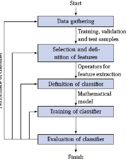
Figure 1.4 shows the principal steps involved in designing a pattern recognition system: data gathering, selection of features, definition of the classifier, training of the classifier, and evaluation. Every step is prone to making different types of errors, but the sources of these errors can broadly be sorted into four categories:

1. Too small a dataset,

2. A non-representative dataset,

3. Inappropriate, non-discriminative features, and

4. An unsuitable or ineffective mathematical model of the classifier.

Fig. 1.4. Design phases of a pattern recognition system.

The following section will describe the different steps in detail, highlighting the challenges faced and pointing out possible sources of error.

(27)

labeled S and consists of patterns of objects where the corresponding classes are known a priori, for example because the objects have been labeled by a domain expert. As the class of each sample is known, deriving a classifier from S constitutes supervised learning. The complement to supervised learning is unsupervised learning, where the class of the objects in S is not known and the goal is to uncover some latent structure in the data. In the context of pattern recognition, however, unsupervised learning is only of minor interest.

A common mistake when gathering the dataset is to pick pathological, characteristic samples from each class. At first glance, this simplifies the following steps, because it seems easier to determine the discriminative features. Unfortunately, these seemingly discriminative features are often useless in practice. Furthermore, in many situations, the most informative samples are those that represent edge cases. Consider a system where the goal is to pick out defective products. If the dataset only consists of the most perfect samples and the most defective samples, it is easy to find highly discriminative features and one will assume that the classifier will perform with high accuracy. Yet in practice, imperfect, but acceptable products may be picked out or products with a subtle, but serious defect may be missed. A good dataset contains both extreme and common cases. More generally, the challenge is to obtain a dataset that is representative of the underlying distribution of classes. However, an unrepresentative dataset is often intentional or practically impossible to avoid when one of the classes is very sparsely populated but representatives of all classes are needed. In the above example of picking out defective products, it is conceivable that on average only one in a thousand products has a defect. In practice, one will select an approximately equal number of defective and intact products to build the dataset S. This means that the so called a priori distribution of classes must not be determined from S, but has to be obtained elsewhere.

Fig. 1.5. Rule of thumb to partition the dataset into training, validation and test sets.

The dataset is further partitioned into a training set , a validation set , and a test set . A rule of thumb is to use 50 % of for , 25 % of for , and the remaining 25 % of for (see Figure 1 .5). The test set is held back and not considered during most of the design process. It is only used once to evaluate the classifier in the last design step (see Figure 1.4). The distinction between training and validation set is not always necessary. The validation set is needed if the classifier in question is governed not only by parameters that are estimated from the training set D, but also depends on so called design parameters or hyper parameters. The optimal design parameters are determined using the validation set.

(28)

point where carrying out the remaining design phases is no longer reasonable. Chapter 9 will suggest methods for dealing with small datasets.

The second step of the design process (see Figure 1.4) is concerned with choosing suitable features. Different types of features and their characteristics will be covered in Chapter 2 and will not be discussed at this point. However, two general design principles should be considered when choosing features:

1. Simple, comprehensible features should be preferred. Features that correspond to immediate (physical) properties of the objects or features which are otherwise meaningful, allow understanding and optimizing the decisions of the classifier.

2. The selection should contain a small number of highly discriminative features. The features should show little deviation within classes, but vary greatly between classes.

The latter principle is especially important to avoid the so called curse of dimensionality (sometimes also called the Hughes effect): a higher dimensional feature space means that a classifier operating in this feature space will depend on more parameters. Determining the appropriate parameters is a typical estimation problem. The more parameters need to be estimated, the more samples are needed to adhere to a given error bound. Chapter 6 will give more details on this topic.

The third design step is the definition of a suitable classifier (see Figure 1.4). The boundary between feature extraction and classifier is arbitrary and was already called “blurry” in Figure 1.2. In the example in Figure 2.4c, one has the option to either stick with the features and choose a more powerful classifier that can represent curved decision boundaries, or to transform the features and choose a simple classifier that only allows linear decision boundaries. It is also possible to take the output of one classifier as input for a higher order classifier. For example, the first classifier could classify each pixel of an image into one of several categories. The second classifier would then operate on the features derived from the intermediate image. Ultimately, it is mostly a question of personal preference where to put the boundary and whether feature transformation is part of the feature extraction or belongs to the classifier.

After one has decided on a classifier, the fourth design step (see Figure 1.2) is to train it. Using the training and validation sets D and V, the (hyper-)parameters of the classifier are estimated so that the classification is in some sense as accurate as possible. In many cases, this is achieved by defining a loss function that punishes misclassification, then optimizing this loss function w.r.t. the classifier parameters. As the dataset can be considered as a (finite) realization of a stochastic process, the parameters are subject to statistical estimation errors. These errors will become smaller the more samples are available.

An edge case occurs when the sample size is so small and the classifier has so many parameters that the estimation problem is under-determined. It is then possible to choose the parameters in such a way that the classifier classifies all training samples correctly. Yet novel, unseen samples will most probably not be classified correctly, i.e., the classifier does not generalize well. This phenomenon is called overfitting and will be revisited in Chapter 6.

(29)

second run. Instead, each separate run should use a different test set, which has not yet been seen in the previous design steps. However, in many cases it is not possible to gather new samples. Again, C hapter 9 will suggest methods for dealing with such situations.

1.5 Exercises

(1.1) Let S be the set of all computer science students at the KIT. For x, y∈ S, let x∼y be true iff x and y are attending the same class. Is x∼y an equivalence relation?

(1.2) Let S be as above. Let x∼y be true iff x and y share a grandparent. Is x∼y an equivalence relation?

(1.3) Let x, y∈ d. Is x ∼ y ⇔ xT y = 0 an equivalence relation?

(1.4) Let x, y∈ d. Is x ∼ y ⇔ xT y ≥ 0 an equivalence relation?

(1.5) Let x, y∈ and f: ↦ be a function on the natural numbers. Is the relation x∼y⇔f(x) ≤f(y) an equivalence relation?

(1.6) Let A be a set of algorithms and for each X∈ A let r(X,n) be the runtime of that algorithm for an input of length n. Is the following relation an equivalence relation?

X∼Y⇔r(X,n) ∈ O (r(Y,n)) for X, Y∈ A.

Note: The Landau symbol O (“big O notation”) is defined by

O (f(n)) := {g(n) | ∃α> 0∃n₀> 0∀n≥n₀: |g(n)| ≤α|f(n)|},

(30)

2 Features

A good understanding of features is fundamental for designing a proper pattern recognition system. Thus this chapter deals with all aspects of this concept, beginning with a mere classification of the kinds of features, up to the methods for reducing the dimensionality of the feature space. A typical beginner’s mistake is to apply mathematical operations to the numeric representation of a feature, just because it is syntactically possible, albeit these operations have no meaning whatsoever for the underlying problem. Therefore, the first section elaborates on the different types of possible features and their traits.

2.1 Types of features and their traits

In empiricism, the scale of measurement (also: level of measurement) is an important characteristic of a feature or variable. In short, the scale defines the allowed transformations that can be applied to the variable without adding more meaning to it than it had before. Roughly speaking, the scale of measurement is a classification of the expressive power of a variable. A transformation of a variable from one domain to another is possible if and only if the transformation preserves the structure of the original domain.

Table 2.1 shows five scales of measurement in conjunction with their characteristics as well as some examples. The first four categories—the nominal scale, the ordinal scale, the interval scale, and the ratio scale—were proposed by Stevens [1946]. Lastly, we also consider the absolute scale. The first two scales of measurement can be further subsumed under the term qualitative features, whereas the other three scales represent quantitative features. The order of appearance of the scales in the table follows the cardinality of the set of allowed feature transformations. The transformation of a nominal variable can be any function f that represents an unambiguous relabeling of the features, that is, the only requirement on f is injectivity. At the other end, the only allowed transformation of an absolute variable is the identity.

2.1.1 Nominal scale

The nominal scale is made up of pure labels. The only meaningful question to ask is whether two variables have the same value: the nominal scale only allows to compare two values w.r.t. equivalence. There is no meaningful transformation besides relabeling. No empirical operation is permissible, i.e., there is no mathematical operation of nominal features that is also meaningful in the material world.

Table 2.1. Taxonomy of scales of measurement. Empirical relations are mathematical relations that emerge from experiments, e.g., comparing the volume of two objects by measuring how much water they displace. Likewise, empirical operations are mathematical operations that can be carried out in an experiment, e.g., adding the mass of two objects by putting them together, or taking the ratio of two masses by putting them on a balance scale and noting the point of the

(31)

A typical example is the sex of a human. The two possible values can be either written as “f” vs. “m,” “female” vs. “male,” or be denoted by the special symbols vs. . The labels are different, but the meaning is the same. Although nominal values are sometimes represented by digits, one must not interpret them as numbers. For example, the postal codes used in Germany are digits, but there is no meaning in, e.g., adding two postal codes. Similarly, nominal features do not have an ordering, i.e., the postal code 12345 is not “smaller” than the postal code 56789. Of course, most of the time there are options for how to introduce some kind of lexicographic sorting scheme, but this is purely artificial and has no meaning for the underlying objects.

With respect to statistics, the permissible average is not the mean (since summation is not allowed) or the median (since there is no ordering), but the mode, i.e., the most common value in the dataset.

2.1.2 Ordinal scale

The next higher scale is made of values on an ordinal scale. The ordinal scale allows comparing values w.r.t. equivalence and rank. Any transformation of the domain must preserve the order, which means that the transformation must be strictly increasing. But there is still no way to add an offset to one value in order to obtain a new value or to take the difference between two values.

Probably the best known example is school grades. In the German grading system, the grade 1 (“excellent”) is betterthan 2 (“good”), which is betterthan 3 (“satisfactory”) and so on. But quite surely the difference in a student’s skills is not the same between the grades 1 and 2 as between 2 and 3, although the “difference” in the grades is unity in both cases. In addition, teachers often report the arithmetic mean of the grades in an exam, even though the arithmetic mean does not exist on the ordinal scale. In consequence, it is syntactically possible to compute the mean, even though the result, e.g., 2.47 has no place on the grading scale, other than it being “closer” to a 2 than a 3. The Anglo-Saxon grading system, which uses the letters “A” to “F”, is somewhat immune to this confusion.

(32)

(number of values) between the p and (1 −p)-quantile. Common values for p are p= 0, which results in the range of the data set, and p= 0.25, which results in the inter-quartile range.

2.1.3 Interval scale

The interval scale allows adding an offset to one value to obtain a new one, or to calculate the difference between two values—hence the name. However, the interval scale lacks a naturally defined zero. Values from the interval scale are typically represented using real numbers, which contains the symbol “0,” but this symbol has no special meaning and its position on the scale is arbitrary. For this reason, the scalar multiplication of two values from the interval scale is meaningless. Permissible transformations preserve the order, but may shift the position of the zero.

A prominent example is the (relative) temperature in °F and °C. The conversion from Celsius to Fahrenheit is given by The temperatures 10 °C and 20 °C on the Celsius scale correspond to 50 °F and 68 °F on the Fahrenheit scale. Hence, one cannot say that 20 °C is twice as warm as 10 °C: this statement does not hold w.r.t. the Fahrenheit scale.

The interval scale is the first of the discussed scales that allows computing the arithmetic mean and standard deviation.

2.1.4 Ratio scale and absolute scale

The ratio scale has a well defined, non-arbitrary zero, and therefore allows calculating ratios of two values. This implies that there is a scalar multiplication and that any transformation must preserve the zero. Many features from the field of physics belong to this category and any transformation is merely a change of units. Note that although there is a semantically meaningful zero, this does not mean that features from this scale may not attain negative values. An example is one’s account balance, which has a defined zero (no money in the account), but may also become negative (open liabilities).

The absolute scale shares these properties, but is equipped with a natural unit and features of this scale can not be negative. In other words, features of the absolute scale represent counts of some quantities. Therefore, the only allowed transformation is the identity.

2.2 Feature space inspection

For a well working system, the question, how to find “good,” i.e., distinguishing features of objects, needs to be answered. The primary course of action is to visually inspect the feature space for good candidates.

(33)

Fig. 2.1. Iris flower dataset as an example of how projection helps the inspection of the feature space.

2.2.1 Projections

(34)

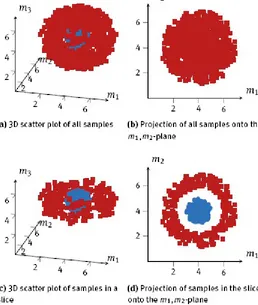
Fig. 2.2. Difference between the full projection and the slice projection techniques.

Figure 2.1a depicts a perspective drawing of the three features petal width, petal length and sepal length. Figure 2.1b shows a two-dimensional projection and two aligned histograms of the same data by omitting the sepal length. The latter clearly shows that the features petal length and petal width are already sufficient to distinguish the species Iris setosa from the others. Further two-dimensional projections might show that Iris versicolor and Iris virginica can also be easily separated from each other.

2.2.2 Intersections and slices

(35)

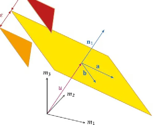
Fig. 2.3. Construction of two-dimensional slices.

The initial situation is depicted in Figure 2.2a. Even though the samples can be separated, any projection to a two-dimensional subspace will suggest that the classes overlap each other, as shown i n Figure 2.2b. However, if one projects slices of the data instead all of it at once, the structure becomes apparent. Figure 2.2c shows the result of such a slice in the three dimensional space and Fig ure 2.2d shows the corresponding projection. The latter clearly shows that one class only encloses the other but can be distinguished nonetheless.

The principal idea of the construction is illustrated in Figure 2.3. The slice is defined by its mean plane (yellow) and a bound ε that defines half of the thickness of the slice. Any sample that is located at a distance less than this bound is projected onto the plane. The mean plane itself is given by its two directional vectors a, b and its oriented distance u from the origin. The mean plane on its own, i.e., a slice with zero thickness (ε= 0), does not normally suffice to “catch” any sample points: If the samples are continuously distributed, the probability that a sample intersected by the mean plane is zero.

Let d∈ be the dimension of the feature space. A two-dimensional plane is defined either by its two directional vectors a and b or as the intersection of d− 2 linearly independent hyperplanes. Hence, let

denote an orthonormal basis of the feature space, where each n_j is the normal vector of a hyperplane. Let u₁, . . . , u_d₋₋₂ be the oriented distances of the hyperplanes from the origin. The two-dimensional plane is defined by the solution of the system of linear equations

(36)

plane in the direction of n_j is given by nT

jm −uj, hence the total Euclidean distance of m from the

plane is

Let m₁, . . . , m_N be the feature vectors of the dataset. Then the two-dimensional projection of the feature vectors within the slice to the plane is given by

2.3 Transformations of the feature space

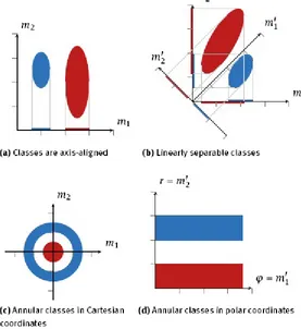
Because the sample size is limited, it is usually advisable to restrict the number of features used. Apart from limiting the selection, this can also be achieved by a suitable transformation of the feature space (see Figure 2.4). In Figure 2.4a it is possible to separate the two classes using the feature m₁

alone. Hence, the feature m₂ is not needed and can be omitted. In Figure 2.4b, both features are needed, but the classes are separable by a straight line. Alternatively, the feature space could be rotated in such a way that the new feature m′_{2 is sufficient to discriminate between the classes. The}

annular classes in Figure 2.4c are not linearly separable, but a nonlinear transformation into polar coordinates shows that the classes can be separated by the radial component. Section 2.7 will present methods for automating such transformations to some degree. Especially the principal component analysis will play a central role.

2.4 Measurement of distances in the feature space

(37)

Fig. 2.4. Feature transformation for dimensionality reduction.

If the feature vector was an element of a standard Euclidean vector space, one could use the well known Euclidean distance

but this approach relies on some assumptions that are generally not true for real-world applications. The cause of this can be summarized by the heterogeneity of the components of the feature space, meaning

– features on different scales of measurement, – features with different (physical) units, – features with different meanings and – features with differences in magnitude.

Above all, Equation (2.5) requires that all components m_i, m′

i, i= 1, . . . , d are at least on an interval

scale. In practice, the components are often a mixture of real numbers, ordinal values and nominal values. In these cases, the Euclidean distance in Equation (2.5) does not make sense; even worse, it is syntactically incorrect.

(38)

The coefficients α₁, . . . , α_d h handle the different units by containing the inverse of the component’s unit, so that each summand becomes a dimensionless quantity. Nonetheless, the question of the difference in size is still an open problem and affords many free design parameters that must be carefully chosen.

Finally, the sum of squares (see Equation (2.5)) is not the only way to merge the different components into one distance value. The first section of this chapter introduces the more general Minkowski norms and metrics. The choice of metric can also influence a classifier’s performance.

2.4.1 Basic definitions

To discuss the oncoming concepts, we must first define the terms that will be used.

Definition 2.1 (Metric, metric space). Let M be a set and m, m′_{, and}_m||||_∈_{M. A function}_D_{: M ×} Kullback–Leibler divergence is not a metric because it lacks the symmetry property and violates the triangle inequality, but it is quite useful nonetheless. Those functions that fulfil some, but not all of the above requirements are usually called distance functions, discrepancys or divergences. None of these terms is precisely defined. Moreover, “distance function” is also used as a synonym for metric and should be avoided to prevent confusion. “Divergence” is generally only used for functions that quantify the difference between probability distributions, i.e., the term is used in a very specific context. Another important concept is given by the term (vector) norm:

Definition 2.2 (Norm, normed vector space). Let M be a vector space over the real numbers and let m, m′_∈_{M. A function ||}_⋅_{|| : M →} ≥0_{is called a}_norm_iff

1. ||m|| ≥ 0 and ||m|| = 0 ⇔ m = 0 (positive definiteness) 2. ||αm|| = |α| m with α∈ (homogeneity)

3. ||_m|| + m′_{≤ ||}_m_{|| + ||}_m′_|| _{(triangle inequality)}

A vector space M equipped with a norm ⋅ is called a normed vector space.

(39)

ratio scale. A norm can be used to construct a metric, which means that every normed vector space is a metric space, too.

Definition 2.3 (Induced metric). Let M be a normed vector space and ⋅ its norm and let m, m′∈ M. Then

defines an induced metric on M.

Note that because of the homogeneity property, Definition 2.2 requires the value to be on a ratio scale; otherwise the scalar multiplication would not be well defined. However, the induced metric from Definition 2.3 can be applied to an interval scale, too, because the proof does not need the scalar multiplication. Of course, one must not say that the metric D(m, m′_{)= ||}_m_-_m′_{|| stems from a}

norm, because there is no such thing as a norm on an interval scale.

2.4.2 Elementary norms and metrics

Inarguably, the most familiar example of a norm is the Euclidean norm. But this norm is just a special embodiment of a whole family of vector norms that can be used to quantify the distance of features on a ratio scale. The norms of this family are called Minkowski norms or p-norms.

Definition 2.4 (Minkowski norm, p-norm) . Let M denote a real vector space of finite dimension

d and let r∈ ∪ {∞} be a constant parameter. Then

is a norm on M.

(40)

Fig. 2.5. Unit circles for Minkowski norms with different choices of r. Only the upper right quadrant of the two-dimensional Euclidean space is shown.

Although r can be any integer or infinity, only a few choices are of greater importance. For r= 2

is the Euclidean norm. Likewise, r= 1 yields the absolute norm

This norm—or more precisely: the induced metric—is also known as taxicab metric or Manhattan metric. One can visualize this metric as the distance that a car must go between two points of a city with a rectilinear grid of streets like in Manhattan. For r= ∞ the resulting norm

is called maximum norm or Chebyshev norm.Figure 2.5 depicts the unit circles for different choices of r in the upper right quadrant of the two-dimensional Euclidean space.

Furthermore, the Mahalanobis norm is another common metric for real vector spaces:

Definition 2.5 (Mahalanobis norm) . Let M denote a real vector space of finite dimension d and let A∈ d×d be a positive definite matrix. Then

is a norm on M.

To a certain degree, the Mahalanobis norm is another way to generalize the Euclidean norm: they coincide for A = I_d. More generally, elements A_iio on the diagonal of A can be thought of as scaling the corresponding dimension i, while off-diagonal elements A_ij, i ≠j assess the dependence between the dimension i and j. The Mahalanobis also appears in the multivariate normal distribution (see Definition 3.3), where the matrix A is the inverse of the covariance Σ of the data.

So far only norms and their induced metrics that require at least an interval scale were considered. The metrics handle all quantitative scales of Table 2.1. The next sections will introduce metrics for features on other scales.

2.4.3 A metric for sets

(41)

or not. However, two sets can also be said to be “nearly equal” when both the intersection and the set difference is non-empty (i.e., they share some, but not all elements). The Tanimoto metric reflects these situations.

Definition 2.6 (Tanimoto metric) . Let U be a finite set, M = P (U) and S₁, S₂∈ M, i.e., S₁, S₂⊆ U. Then

defines a metric on M.

Here, we will omit the proof that D Tanimoto is indeed a metric (interested readers are referred to, e.g., the proof of Lipkus [1999]) and instead investigate its properties. If S₁ and S₂ denote the same set, then |S₁| = |S₂| = |S₁∩ S₂| and therefore D Tanimoto (S1, S2) = 0. Contrary, if S₁ and S₂ do not have any element in common, |S₁∩ S₂| = 0 holds and D Tanimoto (S1, S2) = 1. Altogether, the Tanimoto metric varies on the interval from 0 (identical) to 1 (completely different).

Moreover, the Tanimoto metric takes the overall number of elements into account. Two sets that differ in one element are judged to be increasingly similar, as the number of shared elements

It is not immediately clear how to define a meaningful metric for ordinal features, since there is no empirical addition on that scale. A possible solution is to consider the metric D(m,m′_{) of two ordinal}

features m, m′_{as the number of swaps of neighboring elements in order to reach}_m′_from_m_.

Consider, forexample, the set of characters in the English language {A, B, C, . . . , Z}, where the order corresponds to the position in the alphabet. The metric informally defined above would yield

D(A, C) = 2 and D(A, A) = 0. This example can be generalized as follows:

Definition 2.7 (Permutation metric) . Let M be a locally finite and totally ordered set with a unique successor function, i.e., for each element x∈ M there is a unique next element x′∈ M. Then

is a metric on M.

(42)

Another way to look at Definition 2.7 is to homomorphically map M into the integers (i.e., successive elements of M are mapped to successive integers) and calculate the absolute difference of the numbers corresponding to the sets.

2.4.5 The Kullback–Leibler divergence

The Kullback–Leibler divergence (KL divergence) does not directly quantify a difference between features m, but between probability distributions (characterized by the probability mass function or the probability density) over the features. It is often used as a meta metric to compare objects o_i, i= 1, . . . , N that are in turn characterized by a set of features O_i = {m_j | j= 1, . . . , M_i} }. To this extent, the features in O_i_{are used to estimate the probability mass ̂}P₍_m_{| o}_i₎_{or probability density ̂}p(m | o_i) for each object o_i. The KL divergence is then used to compute the distance between two object-dependent distributions and by proxy the distance between two objects. Here, the ̂P₍_m_{| o}_i₎_{or ̂}p(m | o_i) can themselves be interpreted as features for o_i. An extended example of this approach is given below.

Definition 2.8 (Kullback–Leibler divergence) .

The Kullback–Leibler divergence is not a metric: As can be seen from definition, it is not symmetric and does not obey the triangle inequality. If P′₍_m_{) = 0 and}_P₍_m_{) ≠ 0, one sets}_D₍_P_⇑

P||) = ∞, hence the

range of the KL divergence is [0, ∞]. The Kullback–Leibler divergence is zero if the distributions are equal almost everywhere.

Despite the fact that the Kullback–Leibler divergence is missing important properties of a metric, it is still very useful, because it dominates the difference of the probability density functions with respect to the absolute norm (Minkowski norm with r= 1) by

(43)

The likelihood ratio is the crucial quantity of optimal statistical tests to decide between two competing hypotheses H₁: m∼p(m) and H₂: m∼p′(m) (Neyman and Pearson [1992]). In other words, the Kullback–Leibler divergence measures the mean discriminability between H₁ and H₂.

To become accustomed to the Kullback–Leibler divergence, we will now discuss some simple examples. First, consider the family of Bernoulli distributions parametrized by the probability of success τ∈ [0,1]. That is,

The Kullback–Leibler divergence between two different Bernoulli distributions is therefore given by

Figure 2.6 depicts the value of the Kullback–Leibler divergence as a function of the success probability b of the second distribution while keeping the success probability of the first distribution fixed at a= 0.3.

Now, as an example of the continuous case, consider the Kullback–Leibler divergence of two univariate Gaussian distributions. The Gaussian density function is

Fig. 2.6. Kullback–Leibler divergence between two Bernoulli distributions with fixed success probability a= 0.3 for the first distribution.

(44)

(45)

It is interesting to note that the Kullback–Leibler divergence becomes symmetric if the family of distributions is further restricted to Gaussian distributions with equal variances, i.e., σ2_{1 =}_σ2_{2 =}_σ2_,

i.e., when p₁(m| μ₁,σ), p₂(m| μ₂,σ), one has that D(p₁ p₂)) = D(p₂ p₁). Figure 2.7 shows two pairs of Gaussian distributions with equal variance. The corresponding Kullback–Leibler divergence is noted in the diagram. In order to illustrate the asymmetric behavior of the Kullback–Leibler divergence, Fig ure 2.8 depicts a pair of Gaussian distributions where p_μ1 _σ and p_μ 2, _σ have swapped roles between the diagrams. Once again, the Kullback–Leibler divergence is given in the diagram. As a last example, a pair of rectangle-like densities with unequal support is considered. This example illustrates that the Kullback–Leibler divergence can even take on the value infinity depending on the order of its arguments (see Figure 2.9).

Fig. 2.7. Pairs of Gaussian distributions with equal variance σ2= 0.5 and their KL divergences.

Fig. 2.8. Pairs of Gaussian distribution with different variances and their KL divergences.

(46)

Fig. 2.10. Combustion engine, microscopic image of bore texture and detail with texture model with groove parameters. Source: Krahe and Beyerer [1997].

Extended example: Grading of honing textures

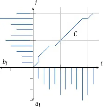
The Kullback–Leibler divergence can be used to derive robust distance measures between features. Consider, for example, the problem of grading honing textures in the cylinder bores of combustion engines, shown in Figure 2.10. This honing texture is the result of a grinding tool rotating around its axis while oscillating inside the cylinder hole. The resulting grooves’ function is to retain lubricant while the pistons move inside the motor block. A single groove in the honing texture is characterized by its amplitude (depth) a and width b. Let further ∆ denote the distance between two given adjacent grooves. From Figure 2.10 it can be seen that the grooves can be divided into two sets, depending on their orientation. The question is: how similar are these sets of grooves?

One possible approach is to model the parameters u := (a,b)T_and_∆_{of the two groove sets}

stochastically. In particular, let us assume that ∆ and u are independent. It is known that the stride ∆

follows an exponential distribution, and it is sensible to assume that the groove depth or amplitude a

and width b are jointly normally distributed. This yields the overall density

Δ Δ

Δ

where i= 1, 2 indicates the first or second set. Here, μ_i is the expected value of u in the i th groove set,

Δ Δ

With ρ_id denoting the correlation coefficient between a_ia and b_i,

Now let C_i be the covariance matrix of u in the i th groove set:

(47)

The parameter λ_id denotes the groove density in the i th set, i.e.,

Δ

This model will be used to construct a measure of the distance between two groove sets. Recall from Definition 2.8 that the KL divergence between p₁ and p₂ is asymmetric. In order to derive a symmetric measure of the distance between two groove sets, we simply take the sum of the KL divergence between p₁ and p₂, and the KL divergence with these arguments transposed:

Δ

Δ Δ

Δ Δ Δ

Δ

Δ Δ

After a fair bit of algebra, this expression simplifies to the sum of three terms:

Δ

This metric can be used to compare two sets of grooves as follows. First, measure the amplitude

a, depth b and distances ∆ of the grooves in the set. Second, estimate the parameters μ_i, C_i and λ_i, i= 1,2 for both sets according to Equations (2.26) to (2.28). Third, compute the distance between the two sets by using Equation (2.30). If the distance is below a given threshold, the honing texture passes the inspection. Otherwise, it is rejected as of insufficient quality.

2.4.6 Tangential distance measure

(48)

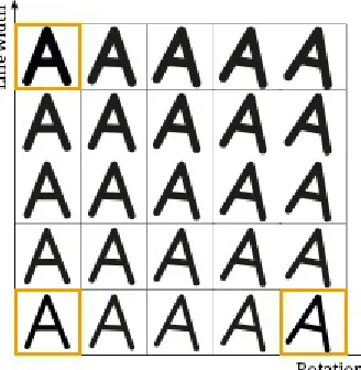
Consider, for example, the problem of optical character recognition. Figure 2.11 shows two possible systematic variations of a character (the pattern): rotation and line thickness. This variation causes differing patterns, and will therefore result in different feature vectors. However, since the variations in the pattern are systematic, so will the variations in the feature vectors. More precisely, small variations of the pattern will move the feature vector within a small neighborhood of the feature vector of the original pattern (given that the feature mapping is smooth in the appropriate sense).

Fig. 2.11. Systematic variations in optical character recognition.

This observation leads the following assumption: The feature vectors O_i = {m_j | j= 1, . . . , M_i} derived from the patterns of an object o_i lie on a topological manifold. The mathematical details and implications of this insight are quite profound and outside the scope of this book. Nonetheless, Appendix B gives a primer of the most important terms and concepts of the underlying theory. For the purposes of this section, it is sufficient to interpret “manifold” as a lower-dimensional hypersurface embedded in the feature space. In other words, the features m_j ∈ O_i of the object o_id do not populate the feature space arbitrarily, but are restricted to some surface within the feature space.

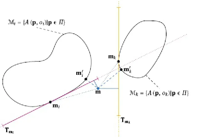
An example is shown in Figure 2.12, where the black curves show the manifolds to which are restricted the features of two objects o_ia and o_k. In the context of the OCR example, the two objects stand for different characters, e.g., o_if for the character “A” and o_kf for the character “B.” Formally, the manifolds are denoted by the set of all points given by an action A of some transformation p on the object o,

Again, the mathematical definitions of the terms are found in Appendix B. Here, it is sufficient to interpret A(p, o_i) as the feature vector that is extracted from some systematic variation parametrized by p.

The Figure 2.12 also highlights an important issue: given a feature vector m to classify and two feature vectors m_i and m_k derived from the objects o_i a and o_k, respectively, computing the distance between the features might lead to the wrong conclusions. Here, m is closest to m_k and hence one could conclude that the object that produced m is more similar to o_k t than to o_i. If, however, one considers the entire manifold of features of both objects, one arrives at a different picture: the closest point to m on M_i (m′