Zhirong Yang1 [email protected]
Jaakko Peltonen1,2 [email protected]
Samuel Kaski1,2,3 [email protected]
1Department of Information and Computer Science, Aalto University, Finland
2Helsinki Institute for Information Technology HIIT, Aalto University and3University of Helsinki
Abstract
Neighbor embedding (NE) methods have found their use in data visualization but are limited in big data analysis tasks due to their O(n2) complexity for n data sam-ples. We demonstrate that the obvious ap-proach of subsampling produces inferior re-sults and propose a generic approximated timization technique that reduces the NE op-timization cost toO(nlogn). The technique is based on realizing that in visualization the embedding space is necessarily very low-dimensional (2D or 3D), and hence efficient approximations developed for n-body force calculations can be applied. In gradient-based NE algorithms the gradient for an in-dividual point decomposes into “forces” ex-erted by the other points. The contributions of close-by points need to be computed indi-vidually but far-away points can be approx-imated by their “center of mass”, rapidly computable by applying a recursive decom-position of the visualization space into quad-rants. The new algorithm brings a significant speed-up for medium-size data, and brings “big data” within reach of visualization.
1. Introduction
Very simple techniques dominate in visual analytics and large-scale information visualization, as the com-putational complexity of advanced nonlinear dimen-sionality reduction (NLDR) methods developed in the machine learning community is too high. There is an immediate need for methods for initial inspection, “looking at the data”, for the sets that typically
cur-Proceedings of the 30th International Conference on
Ma-chine Learning, Atlanta, Georgia, USA, 2013. JMLR:
W&CP volume 28. Copyright 2013 by the author(s).
rently range in tens of thousands or millions of data samples. The scatterplot-type displays produced with NLDR are one of the most common tools for smaller sets and would be useful for the “bigger data” as well.
Neighbor embedding (NE) methods work by optimiz-ing the low-dimensional output coordinates of sam-ples, and some other NLDR methods by optimizing the mapping function. The cost functions typically measure preservation of distances or neighborhood re-lationships from the original space to the output space. Unfortunately, current advanced NLDR methods do not scale well to large data sets, as the computational complexity of their optimization is typically at least quadratic (O(n2) forndata samples), and may be cu-bic or even worse. This is unfeasible for large data sets, and in some cases also the memory complexity may grow unmanageably large. The naive solution, of applying NLDR to a subset of data only, is unsatisfac-tory as it neglects the vast majority of relationships in data. We demonstrate experimentally that the naive solution can lead to poor generalization.
In this paper we present novel, fast and scalable ver-sions of several recent state-of-the-art NE methods, by applying an efficient approximation to their gradient terms. The key insight is that in the methods we con-sider, interactions between far-away data samples do not contribute much to the gradient, and hence their contribution can be computed with stronger approx-imations. Inspired by the Barnes-Hut simulation ap-proach in n-body dynamical systems (Barnes & Hut, 1986), we use a quad-tree to approximate far-away pairwise interactions: for each data sample, the effect of a far-away sample is approximated by the effect of the mean of a hierarchical cluster. The farther away the samples, the less detailed clusters are needed.
(SNE;Hinton & Roweis,2002), t-distributed Stochas-tic Neighbor Embedding (t-SNE; van der Maaten & Hinton, 2008), Elastic Embedding (EE; Carreira-Perpi˜n´an, 2010), and Neighbor Retrieval Visualizer (NeRV;Venna & Kaski,2007;Venna et al.,2010). We show in experiments that our efficient NLDR methods clearly outperform the original state of the art meth-ods in terms of computation time, and achieve essen-tially the same quality. We demonstrate that the new methods bring within reach of visualizations very large data sets which could not be processed in a reasonable time by the existing state-of-the-art methods.
2. Neighbor Embedding
We now present the methods we will make scalable. Neighbor Embedding (NE) is a family of methods for finding a configuration of data points in a lower-dimensional “embedding space”. Given a set of mul-tivariate data points{x1, x2, . . . , xn}, wherexi∈RM, their neighborhood is encoded in a square nonnegative matrixP, wherePij is proportional to the probability thatxj is a neighbor ofxi. Neighbor Embedding finds a mapping xi 7→ yi ∈ Rm for i = 1, . . . , n such that the neighborhoods are approximately preserved in the mapped space. Usually m= 2 or 3, and m < M. If the neighborhood in the mapped space is encoded in
Q∈Rn×n such thatQij is proportional to the prob-ability that yj is a neighbor of yi, the NE task is to minimizeD(P||Q) overY = [y1, y2, . . . , yn]T for a cer-tain divergenceD.
Different choices of P, Q and D give different Neighbor Embedding methods. Let pij ≥ 0 and
qij , q kyi−yjk2 > 0. The NE method Stochas-tic Neighbor Embedding (SNE; Hinton & Roweis, 2002) uses Pij = Ppij
kpik, Qij = qij P
kqik and Kullback-Leibler divergence in the cost function, D(P||Q) =
P
iDKL(Pi:||Qi:). The qij is typically chosen to be proportional to the Gaussian distribution so thatqij = exp −kyi−yjk2, or proportional to the Cauchy dis-tribution so thatqij= (1 +kyi−yjk2)−1.
Additionally bringing in the dual Kullback-Leibler di-vergence DKL(Q||P) weighted by a tradeoff parame-ter λ∈(0,1), hence minimizingP
iλDKL(Pi:||Qi:) + (1−λ)DKL(Qi:||Pi:) overY, results in a method called NeRV. NeRV has an information retrieval interpreta-tion of making a tradeoff between precision and re-call; SNE is a special case (λ= 1) maximizing recall, whereasλ= 0 maximizes precision.
If Pij = Ppij metric SNE (s-SNE). When qij is proportional to the
Cauchy distribution, it is also called t-SNE (van der Maaten & Hinton, 2008; t denotes the Student t -distribution with a single degree of freedom).
If neither neighborhood matrix is normalized and the divergence is the non-normalized Kullback-Leibler di-vergence DI(p||ρq) = Pij
h
pijlogρqpijij −pij+ρqij
i
, with a constant scalarρ >0, the NE method is equiv-alent to the Elastic Embedding (Carreira-Perpi˜n´an, 2010) whenqij is set to be Gaussian. Some additional methods have also been introduced to the NE family, for example, LinLog (Noack,2007) which uses Itakura-Saito divergence and HSSNE (Yang et al.,2009) which uses other heavy-tailed embedding functions. We skip their description to avoid notational clutter.
We make the common approximation of sparsifying
P by zeroing the very small non-local input similari-ties. This makes sense for two reasons: 1) geodesics of curved manifolds in high-dimensional spaces can only be approximated by Euclidean distances in small neighborhoods; 2) most popular distances computed of weak or noisy indicators are not reliable over long distances. The matrix P is often built upon the k -nearest-neighbor graph, of which there exist various efficient construction methods (see e.g.Yianilos,1993; Liu et al.,2004;Beygelzimer et al.,2006). Note that in general the output similarity matrixq(orQ) is dense. The costly computation of this part can be avoided by using the technique described in the next section.
3. Scalable Optimization for NE
The neighbor embedding methods in Section 2 have an objectiveJ and partial derivative ∂J∂yi of the form
J =
the whole data, rather it embeds a reduced and blurred neighborhood among the subset. In addition, comput-ing the multi-path connections is expensive.
Fast group-based approximation. We propose an approximation method to speed up the objective and gradient calculation in NE. The computational com-plexity in NE is essentially due to the coordinates and pairwise distances in the output space, which change at every step of optimization. The idea is that, in each complicated sum computed around a data point
i in the output space (each sum over neighbors j of the point), the terms in the sum will be partitioned into several groupsGi
tand each group will be approxi-mated as an interaction with a representative point of the group. Consider the following summation which appears commonly in NE objectives:
X
whereiis the starting data point,j are its neighbors,
Gi
tare groups (subsets) of the neighborsj,|Git|is the size of the group, and ˆyi
t is the representative, e.g. mean, of the points in group Gi
t. Similarly, we can approximate the gradient of the above sum. Denote
gij =f′ kyi−yjk2. We have
The approximation within each group Gi
t is accurate when all points in the group are far enough from yi. Otherwise we divide the group into subgroups and re-cursively apply the approximation principle to each subgroup, until the group contains a single point j
where we directly calculatef kyi−yjk2orgij. This grouping hierarchy forms a tree-like structure. In prac-tice, the tree does not need to be constructed sepa-rately around each pointi; it is enough to use a single global tree. We thus omit the superscriptiin what fol-lows. Summations of O(n) cost can be approximately calculated inO(logn) time if each split in the tree di-vides the data into roughly equal size parts.
Fast computation of Eqs.3 and4suffices to speed up methods with pairwise separable NE objectives such as Elastic Embedding. For NE methods involving nor-malized similarities, each normalizing denominator is another sum which can be approximated before com-putation of the cost function or gradient using the
same principle. Some methods like NeRV need inner summations in the objective or gradient, which can be approximated beforehand in the same way.
Tree construction. The above approximation orig-inated in the n-body problem in physics, where fast computation of energy (objective) and forces (gradi-ent) is needed to study systems with huge numbers of particles. Various hierarchical structures exist for the speedup, e.g. fast multipole method (Greengard & Rokhlin, 1987) and dual tree (Gray & Moore, 2001; 2003a;b). We choose the one byBarnes & Hut (1986) as it is simple. The cost of building such a tree is neg-ligible compared to computation time of the NE ob-jective or gradient. For notational brevity we only de-scribe Barnes-Hut QuadTree for two dimensional out-put points; it is straightforward to extend the principle to the three dimensional case (OctTree).
A QuadTree is constructed as follows. First the root node is assigned the smallest bounding box that con-tains all data points, and a representative which is the mean of all points. If the bounding box contains more than one data point, it is divided into four smaller boxes of equal size, and a child node is constructed at each smaller bounding box if it contains at least one data point. The splitting is done recursively until all leaf nodes contain exactly one data point.
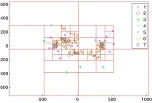
Fig.1shows an example QuadTree. Note that the tree respects point density—an area with more data points is split into deeper levels. Each tree node contains a group of data points. LetGt denote the set of points within the bounding box in a branch (non-leaf) node
t. The branch node also has the following data fields: a position ˆytwhich is the mean of points inGt, and a weight |Gt| which equals the size of Gt. An optional coefficient may also be attached to a branch node to facilitate computation (e.g. to precompute means of some functions over the groups, needed for methods like NeRV). The memory cost of a QuadTree is thus linear in the number of data points.
Using the tree in computation. What remains is to define a criterion that a pointyiis far from a treet. A straightforward idea is that the tree’s bounding box is small enough compared to the distance kyi−yˆtk. This can be implemented by
θ·TreeWidth(t)<kyi−yˆtk, (5)
Figure 1.An example QuadTree for 62 data points. The color labeling corresponds to the depth of each data point.
As an example, we show how to apply the approxima-tion to t-SNE. Again denote the objective byJ. The t-SNE gradient is ∂J and then further approximate the gradient by Eq. 4. This suffices for algorithms that only need gradients. For those which use line search, the objective can also be cheaply obtained: J ≈P
ijPijkyi−yjk
2+ log ˆs+
constant, where ˆs is the approximation of s and we compute the first term by exploiting sparsity ofP.
4. Experiments
We experimentally verify the performance of the al-gorithm, and demonstrate that alternative speedups are not comparable. The experiments were run on sixteen publicly available datasets (details in the sup-plemental document). For NE, each data set was con-verted to a symmetrized k-Nearest Neighbor matrix (k-NN; k = 10 in all reported results) with pij = 1 if j is among k nearest neighbors of i or vice versa, and pij = 0 otherwise. Conclusions are the same for
k= 15 andk= 20, and for Gaussian kernel matrices.
4.1. More data in NE learning helps
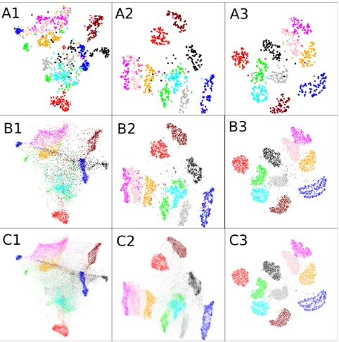
We first test how well the straightforward fast alter-native of subsampling and interpolation would per-form. We compute the embedding for only a random subset of data, and then interpolate the rest in with Locality-constrained Linear Coding (Wang et al.,2010; Carreira-Perpi˜n´an,2010presented another method for out-of-sample extension, which is however restricted to the EE method and requires expensive iterative learn-ing). The result of embedding a 700-point subset of the 70,000 digit images from the MNIST data is shown in A1 of Figure 2, and with all points interpolated in C1. When compared to the optimal visualization com-puted for all the 70,000 points in C3, it is clear that the interpolation misses and mixes up a lot of the structure in the data.
One might argue that the smaller subset is already sufficiently large to give an overview of the whole set, and hence the larger visualization is not needed. In A3 the same small set of 700 points is shown, but on the display optimized for all the 70,000 points. The visualization reveals the classes and cluster structure much clearer than A1 which has been computed only on the small set.
The conclusion is that learning the visualizations on large data is beneficial, irrespective of whether only a subset or all data are to be visualized. The remaining problem is that embeddings with the largest data are expensive to compute: generating subfigure C3 takes about 46 hours. With the new algorithms a visual-ization of almost the same quality can be achieved in around 1.6 hours (Fig.4A).
4.2. Learning speed comparison
We tested the speed-up produced by the new approx-imation technique on three NE methods: t-SNE, s-SNE with Spectral Direction (SD) optimization ( Vla-dymyrov & Carreira-Perpi˜n´an,2010), and s-SNE with momentum optimization (van der Maaten & Hinton, 2008). We will refer to the original ones byexact algo-rithms and the new ones byapproximated algorithms.
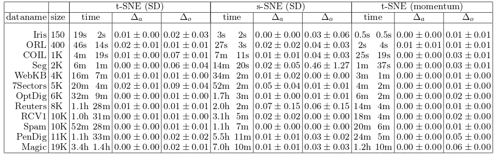
First we compared the learning times. Each method was run for each dataset ten times, stopping when kYnew−Yk
F <10−6·kYkF or the number of iterations exceeded 1000. To keep these computations manage-able, only data sets with less than 20,000 samples were included. A clear speedup was obtained on all the data sets in terms of the mean elapsed times (Table1).
We then verified that the approximated algorithms produce embeddings of comparable quality to the ex-act ones. We measured the quality with two quanti-ties: relative difference ∆obetween the objective func-tion values and relative difference ∆a in the 10-NN classification accuracies (A) computed after the em-bedding: ∆o = |Jexact− Japprox|/|Jexact| and ∆a = |Aexact− Aapprox|/|Aexact|. The measures are gener-ally close to zero (Table1), except for one dataset on s-SNE (SD). This indicates the approximation accu-racy by using the proposed technique is satisfactory.
Table 1.Effects of the new approximations on three NE methods, with 12 data sets. In each time column, the first figure is the elapsed time of the original (exact) algorithm and the second the approximated algorithm (“s”:second, “m”:minute, “h”:hour). ∆o: relative difference in objective function values (±standard deviation); ∆a: relative difference in k-NN
classification accuracy on the display.
t-SNE (SD) s-SNE (SD) t-SNE (momentum) dataname size time ∆a ∆o time ∆a ∆o time ∆a ∆o
Iris 150 19s 2s 0.01±0.00 0.02±0.03 3s 2s 0.00±0.00 0.03±0.06 0.5s 0.5s 0.00±0.00 0.01±0.01 ORL 400 46s 14s 0.02±0.01 0.01±0.01 27s 3s 0.02±0.02 0.04±0.03 2s 4s 0.01±0.01 0.01±0.01 COIL 1K 4m 19s 0.01±0.00 0.07±0.01 7m 11s 0.01±0.01 0.04±0.03 25s 19s 0.00±0.00 0.03±0.01 Seg 2K 6m 1m 0.00±0.00 0.06±0.04 14m 20s 0.02±0.05 0.46±1.27 1m 37s 0.00±0.00 0.03±0.01 WebKB 4K 16m 7m 0.01±0.01 0.01±0.00 34m 2m 0.01±0.02 0.00±0.00 3m 1m 0.00±0.00 0.01±0.00 7Sectors 5K 20m 4m 0.02±0.01 0.09±0.04 52m 2m 0.05±0.04 0.01±0.01 4m 2m 0.00±0.00 0.01±0.00 OptDig 6K 32m 9m 0.00±0.00 0.01±0.00 1.7h 3m 0.01±0.00 0.01±0.01 6m 2m 0.00±0.00 0.02±0.00
Reuters 8K 1.1h 28m 0.01±0.00 0.01±0.01 2.0h 2m 0.07±0.15 0.06±0.15 14m 4m 0.00±0.00 0.01±0.00
RCV1 10K 1.0h 31m 0.00±0.01 0.01±0.00 3.1h 5m 0.02±0.02 0.00±0.00 18m 4m 0.00±0.00 0.02±0.00
Spam 10K 52m 28m 0.00±0.00 0.01±0.01 1.1h 7m 0.00±0.00 0.00±0.00 20m 6m 0.00±0.00 0.01±0.00
PenDig 11K 1.1h 33m 0.00±0.00 0.02±0.02 5.5h 11m 0.01±0.01 0.03±0.02 24m 5m 0.00±0.00 0.05±0.00
Magic 19K 3.4h 1.4h 0.00±0.00 0.02±0.01 7.0h 10m 0.01±0.01 0.03±0.03 1.2h 10m 0.00±0.00 0.06±0.00
4.3. Comparison to workaround in van der Maaten & Hinton(2008)
We compared the efficiency of our approach against another approximation approach (landmark t-SNE) by van der Maaten & Hinton (2008) on the MNIST dataset. The landmark t-SNE also starts from a sparse similarity input, for example k-NN. Differently, they first sample a subset of landmarks from the whole dataset, and then they calculate the similarities among the landmarks by considering multi-path connections, which is implemented with random walk smoothing. Finally a much smaller matrix is fed to t-SNE and only the landmarks will be displayed.
Landmark t-SNE has a number of drawbacks. In appli-cation, it cannot visualize the whole dataset. There-fore, it can only discover a macro structure for cer-tain datasets, given that the structure coincides with the blurring distortion by random walk. In terms of computational cost, landmark t-SNT requires solving a very large linear system to find the multipath similar-ities between the landmarks. In our practice, finding a solution for the MNIST data costs 6-10 hours in a machine with an Intel Core i7 CPU. For even larger datasets, e.g. UCI Covertype and TIMIT in Section 4.4, landmark t-SNE causes out-of-memory failure.
In contrast, the approximated version of t-SNE with SD only takes about 1.6 hours, with small memory cost but an even better visualization (Section 4.4).
4.4. Visualization of large data
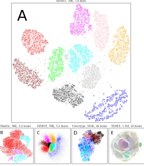
We finally demonstrate with the visualizations in Fig-ure4that the new fast methods make feasible embed-ding of very large data sets. Subfigure A visualizes 70,000 digit images from MNIST by the approximated t-SNE with SD optimization. The classes are well
sep-arated and the plot is almost as good as exact t-SNE in Figure 2 (C3), even though the computation time has been reduced from 46 hours to 1.6 hour. Subfigure B shows 58,000 points from the UCI Shuttle data (7 classes of shuttle states) embedded by approximated s-SNE with SD optimization; the classes are well ar-ranged with sharp borders. SubfigureCshows our ini-tial results with a fast NeRV by SD optimization on the MNIST data; classes are well arranged although some class overlap is visible. Subfigure D shows 581,012 points from the UCI Covertype data (7 classes of for-est cover types) embedded by s-SNE with SD; clear structure is visible and classes are locally well arranged although complete class separation is not easy for this challenging data. SubfigureEshows 1.3 million points from the DARPA TIMIT acoustic speech database (points are 39ms segments with MFCC features; 49 phoneme classes) embedded by approximated t-SNE with momentum optimization; although full class sep-aration is not easy for the hard TIMIT data, clear structure is again visible and there are several local areas where classes are separated. Especially the visu-alizations of TIMIT and Covertype would take unfea-sibly long with the exact methods.
Overall, the fast methods can embed very large data sets quickly. Even though the methods are unsuper-vised, the arrangements revealed hidden ground truth classes well. Even more importantly, the methods made visualization possible for huge data sets where the original exact methods would have been infeasible.
4.5. The θ parameter
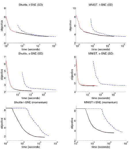
gener-MNIST, 70K, 1.6 hour
Shuttle, 58K, 3.2 hours MNIST, 70K, 5.4 hours Covertype, 581K, 46 hours TIMIT, 1.3M, 33 hours
Figure 3.Speedup on three methods (rows) for two large data sets (columns). The curves show the evolution of the objective function value as a function of time for the exact algorithm (dash-dotted line) and approximated algorithm (dashed line). The solid line shows the (off-line computed) value of the exact cost function for the solution produced by the approximated algorithm. For momentum optimiza-tion, both dash and solid lines are offline calculated.
ated a 2D mapping by normal distribution with vari-ance uniformly from [10−10,1010]. The resulting ap-proximated objective and gradient is compared with the exact ones. Their relative differences are mea-sured by ∆o = |Jexact− Japprox|/|Jexact| and ∆g = k∇exact− ∇approxkF/k∇exactkF, respectively, where∇ stands for the gradient. We ran the experiment 10 times and recorded the mean and standard deviation.
The results are shown in Figure 5. We can see that relative differences vanish quickly with increasing θ. Whenθ >5, more computational cost brings little ac-curacy improvement. The phenomenon holds for both the objective and gradient. The above experiments in-dicate that generally a smallθis enough for NE meth-ods such as t-SNE or s-SNE. A relatively largerθ can be used for more complicated methods which require several levels of approximation, for example, NeRV.
5. Conclusions
We have introduced novel fast versions of neighbor em-bedding methods where interactions to far-away points are approximated at centers-of-mass of a hierarchical
Figure 5.Relative differences between the exact and ap-proximated (left) objectives and (right) gradients across variousθ values.
quad-tree, yielding fastO(nlogn) complexity for cost function and gradient computation. With this ap-proach we created fast versions of Stochastic Neighbor Embedding (SNE), symmetric SNE, andt-distributed SNE; the same approach also yields fast algorithms for Elastic Embedding and the Neighbor Retrieval Visu-alizer which we did not focus on here.
We demonstrated that embedding large data helps even if only a subset is ultimately plotted, and that the straightforward approach of embedding a subset and bringing in the other data by interpolation does not work well. We showed on several benchmark data sets that our fast methods can embed the full data with minimal difference in quality (measured by cost functions of the original methods and by classifica-tion accuracy) and in far less time. We then demon-strated our methods on very large data up to 1.3 mil-lion points. Overall, our fast methods make it feasible to visualize “big data” by advanced nonlinear embed-ding approaches. Our NE software can be found in http://research.ics.aalto.fi/mi/software/ne/.
Interestingly, the Barnes-Hut approximation that we used to derive our fast methods has previously been applied in another genre, graph drawing methods, but to our knowledge not for visualizing manifold data. Our results show that state-of-the-art manifold learn-ing methods can greatly benefit from our fast compu-tation approach with very little loss of quality.
The experiments in this work have been performed in a single-core setting. Our method, however, does not prevent distributed implementations using modern parallel computing tools such as GPU or MapReduce. QuadTree as the only centralized component is linear in the number of data points in 2D or 3D. For even larger datasets, one may consider distributed hash ta-bles (e.g.Miller et al.,2010) to de-centralize the tree.
Acknowledgment
References
Barnes, J. and Hut, P. A hierarchical O(N log N) force-calculation algorithm.Nature, 324(4):446–449, 1986.
Beygelzimer, A., Kakade, S., and Langford, J. Cover trees for nearest neighbor. In International Con-ference on Machine Learning (ICML), pp. 97–104, 2006.
Carreira-Perpi˜n´an, M. The elastic embedding algo-rithm for dimensionality reduction. InInternational Conference on Machine Learning (ICML), pp. 167– 174, 2010.
Gray, A. and Moore, A. N-body problems in statis-tical learning. In Advances in Neural Information Processing Systems (NIPS), pp. 521–527, 2001.
Gray, A. and Moore, A. Rapid evaluation of mul-tiple density models. In International Conference on Artificial Intelligence and Statistics (AISTATS), 2003a.
Gray, A. and Moore, A. Nonparametric density es-timation: toward computational tractability. In
In SIAM International Conference on Data Mining (ICDM), 2003b.
Greengard, L. and Rokhlin, V. A fast algorithm for particle simulations. Journal of Computational Physics, 73(2):325–348, 1987.
Hinton, G.E. and Roweis, S.T. Stochastic neighbor embedding. InAdvances in Neural Information Pro-cessing Systems (NIPS), pp. 833–840, 2002.
Liu, T., Moore, A., Gray, A., and Yang, K. An in-vestigation of practical approximate nearest neigh-bor algorithms. InAdvances in Neural Information Processing Systems (NIPS), pp. 825–832, 2004.
Miller, F.P., Vandome, A.F., and McBrewster, J. Dis-tributed Hash Table. Alphascript Publishing, 2010.
Noack, A. Energy models for graph clustering.Journal of Graph Algorithms and Applications, 11(2):453– 480, 2007.
van der Maaten, L. and Hinton, G. Visualizing data us-ing t-SNE. Journal of Machine Learning Research, 9:2579–2605, 2008.
Venna, J. and Kaski, S. Nonlinear dimensionality re-duction as information retrieval.Journal of Machine Learning Research - Proceedings Track, 2:572–579, 2007.
Venna, J., Peltonen, J., Nybo, K., Aidos, H., and Kaski, S. Information retrieval perspective to non-linear dimensionality reduction for data visualiza-tion. Journal of Machine Learning Research, 11: 451–490, 2010.
Vladymyrov, M. and Carreira-Perpi˜n´an, M. Partial-hessian strategies for fast learning of nonlinear em-beddings. In International Conference on Machine Learning (ICML), pp. 167–174, 2010.
Wang, J., Yang, J., Yu, K., Lv, F., Huang, T., and Gong, Y. Locality-constrained linear coding for im-age classification. InIEEE Conference on Computer Vision and Pattern Recognition (CVPR), pp. 3360– 3367, 2010.
Yang, Z., King, I., Xu, Z., and Oja, E. Heavy-tailed symmetric stochastic neighbor embedding. In Ad-vances in Neural Information Processing Systems (NIPS), volume 22, pp. 2169–2177, 2009.