RANDOM-FOREST-ENSEMBLE-BASED CLASSIFICATION OF HIGH-RESOLUTION
REMOTE SENSING IMAGES AND NDSM OVER URBAN AREAS
X. F. Sun a, X. G. Lin a, *
a
Institute of Photogrammetry and Remote Sensing, Chinese Academy of Surveying and Mapping, No. 28, Lianhuachixi Road, Haidian District, Beijing 100830, China - [email protected], [email protected]
KEY WORDS: Semantic labelling, Random forest, Conditional random field, Differential morphological profile, Ensemble learning.
ABSTRACT:
As an intermediate step between raw remote sensing data and digital urban maps, remote sensing data classification has been a challenging and long-standing research problem in the community of remote sensing. In this work, an effective classification method is proposed for classifying high-resolution remote sensing data over urban areas. Starting from high resolution multi-spectral images and 3D geometry data, our method proceeds in three main stages: feature extraction, classification, and classified result refinement. First, we extract color, vegetation index and texture features from the multi-spectral image and compute the height, elevation texture and differential morphological profile (DMP) features from the 3D geometry data. Then in the classification stage, multiple random forest (RF) classifiers are trained separately, then combined to form a RF ensemble to estimate each sample’s category probabilities. Finally the probabilities along with the feature importance indicator outputted by RF ensemble are used to construct a fully connected conditional random field (FCCRF) graph model, by which the classification results are refined through mean-field based statistical inference. Experiments on the ISPRS Semantic Labeling Contest dataset show that our proposed 3-stage method achieves 86.9% overall accuracy on the test data.
*Corresponding author.
1. INTRODUCTION
Remote sensing data classification has been a challenging and long-standing research problem in the community of remote sensing. As an intermediate step between raw remote sensing data and digital urban maps, its aim is to determine, at any spatial position of urban areas, the most likely class label among a finite set of possible labels, corresponding to the desired object categories in the map (Marmanis et al., 2016). Despite decades of research, the degree of automation for map generation and updating still remains low. In practice, most maps are still drawn manually, with varying degree of support from semi-automated tools (Helmholz et al., 2012).
The existing methods for remote sensing data classification can be categorized into different groups based on different criterion. Based on the types of data sources employed, the existing methods can be categorized into image based classification, 3D point cloud based classification and data fusion based classification. Image based classification only makes use of the available multi-spectral or hyper-spectral image as the sole data source in classification, as done in (Lu et al., 2014; Benediktsson et al., 2005). 3D point cloud acquired by light detection and ranging (LIDAR) or some image dense matching techniques (Shen, 2013; Furukawa and Ponce, 2013) is another effective data source for remote sensing data classification. For example, Vosselman (Vosselman, 2013) used high density point clouds of urban scenes to identify buildings, vegetation, vehicles, ground, and water. Zhang et al. (Zhang et al., 2013) used the geometry, radiometry, topology and echo characteristics of airborne LIDAR point cloud do an object-based classification. To exploit the complementary characteristics of multi-source data, data fusion based methods are also popular and have been proved to be more reliable than the single-source data based ones by many researchers (Zhang
and Lin, 2016). For example, both images and 3D geometry data were used in (Rau et al., 2015; Gerke and Xiao, 2014; Khodadadzadeh et al., 2015; Zhang et al., 2015).
According to the basic element employed in classification process, the existing methods can be categorized into segmentation-based ones and segmentation-free-based ones. Segmentation-based methods typically use a cascade of bottom-up data segmentation and region classification, which makes the system commit to potential errors of the front-end segmentation system (Chen et al., 2015). For instance, Gerke (Gerke, 2015) first segmented the image into small super-pixels, then features of each super-pixel are extracted and inputted to an AdaBoost classifier for classification; Zhang et al.( Zhang et al., 2013) first grouped point cloud into segments by a surface growing algorithm, then classified the segments by a support vector machine (SVM) classifier. Segmentation-free-based methods leave out the segmentation process and directly classify each pixel/point. However, duo to the lack of contextual information, the classified results usually seem noisy; as a kind of remedial measures, a conditional random field (CRF) is usually used to smooth the classification result. For example, both Marmanis et al. (Marmanis et al., 2016) and Paisitkriangkrai et al. (Paisitkriangkrai, 2015) used deep convolutional neural networks (CNN) classify each pixel, then CRF were used to refine the results; whereas Niemeyer et al. (Niemeyer et al., 2013) first classified each 3D point by a random forest (RF) classifier then smoothed them by CRF.
In terms of the classifiers used, the existing methods can be divided into two types: unsupervised ones and supervised ones. For the unsupervised method, some expert knowledge for each class is usually summarized and used to classify the data into different categories. For instance, a rule-based hierarchical classification scheme that utilizes spectral, geometry and topology knowledge of different classes was used by both Rau
Commission III, WG III/6
et al. (Rau et al., 2015) and Speldekamp et al. (Speldekamp et al. 2015) for classifying different data. As for the supervised methods, some samples with labeled ground truth are first used to train a statistical classifier (e.g. AdaBoost, SVM and RF), then the samples without labels are classified by this learned classifier. Previously, samples from small areas were usually used to train the classifier and features of these samples were all designed manually (Zhang and Lin, 2013; Niemeyer et al., 2013; Wei et al., 2012). More recently, with the progress of sensor technology, an increasing number of high quality remote sensing data is available for researching. At the same time progresses in graphic processing unit (GPU) and parallel computing technology significantly increase the computing capability, such that learning a more complicated classifier with larger amount of training data becomes accessible to commoners. Specifically, one of the most successful practices in this direction is the deep CNN (Krizhevsky et al., 2012; Sermanet et al., 2014; Simonyan and Zisserman, 2013; He et al., 2016) launched in the computer vision community which has become the dominant method for visual recognition, semantic classification, etc (Chen, 2015; Sherrah, 2016; Lin et al., 2016; Long et al., 2015; Papandreou et al., 2015). Furthermore, one of the most distinct characteristics of CNN is its ability to learn the most suitable features by itself and this made the hand-crafted feature extraction process used in the traditional supervised-based classification methods unnecessary. However, comparing to the data used in the semantic classification task in computer vision community, remote sensing data usually has a great difference. Although some researches (Paisitkriangkrai et al., 2015; Penatti et al., 2015) found that the CNN models trained by computer vision community generalize well in remote sensing and the features learned by them were more discriminative than the hand-crafted features, we found that compared with the traditional methods the superiority of CNN is not as significant as in computer vision community. In this work, we explore that whether the limited gap between traditional method and CNN can be further reduced with the aid of large-scale training data.
It is widely held that for CNN-based methods, the more training data are available, the more benefits could be gained. However, different from CNN, too many training samples may lead to disaster for some traditional supervised classifiers. For example, if SVM was trained by a large-scale dataset, it often suffers from large memory storage and time consuming problem. Since a SVM solver should solve a complex dual quadratic optimization problem (Ravinderreddy et al., 2014). Besides, the existence of too many support vectors will make the solving process extremely slow (Hsu and Lin, 2002). Although the RF and AdaBoost classifiers can theoretically handle a large-scale dataset, the large memory storage and computational load still hamper their applications in big training data. It is for tackling this problem and taking full advantage of the information existed in the large-scale dataset, we introduced the RF-based ensemble learning strategy in this work. Ensemble learning or multiple classifier system (MCS) is well established in remote sensing and has shown great potential to improve the accuracy and reliability of remote sensing data classification over the last two decades (Du et al., 2012; Lu and Weng, 2007; Briem et al., 2002). For example, Waske et al. (Waske and Benediktsson, 2007) fused two SVM classifiers for classifying both the optical imagery and synthetic aperture radar data, each data source was treated separately and classified by an independent SVM. Experiments showed that their fusion method outperforms many approaches and significantly improves the results of a single SVM, which was trained on the whole multisource dataset. Ceamanos et al. (Ceamanos and Waske, 2010) designed a
classifier ensemble for classifying hyper-spectral data. Spectral bands of hyper-spectral image were first divided into several sub-groups according to their similarity. Then, each group was used for training an individual SVM classifier. Finally an additional SVM classifier was used to combine these classifiers together. The results also demonstrated the effectiveness of their model fusion scheme.
In our work, the remote sensing data (both the multi-spectral image and 3D geometry data) is first divided into tiles. Then, some of them are selected and labeled by a human operator. After that, each selected and labeled tile is used for training an individual RF model. Finally, a Bayesian weighted average method (Du et al., 2012) is employed to combine these individual RF models as a global classifier. In addition, for taking full advantage of the contextual information in the data, an effective fully connected conditional random field (FCCRF) model is constructed and optimized to refine the classified results.
2. THE PROPOSED METHOD
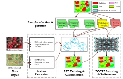
Our proposed method consists of three main parts: first, both the high-resolution multi-spectral image and the 3D geometry data are used for feature extraction, and totally 24 different features are extracted for each pixel; second, using these pixels (samples), an RF ensemble model (constructed by combining several individual RF models; denoted by RFE) is trained and used to classify the scene; finally, the noisy classification results are inputted to a learned FCCRF model, and a long-range dependencies inference is used to refine the classification result. Figure 1 shows the pipeline of the proposed method.
· Different color spaces
Figure 1. Pipeline of the proposed classification method.
2.1. Feature Extraction
Three types of features are employed in this work, which are: spectral features from the multi-spectral image, texture features from the multi-spectral image and geometry features from the 3D geometry data.
2.1.1. Spectral Features
The spectral features used in this paper refer to two types: features in different color spaces and vegetation index. They are defined as below.
1) Features in different color spaces. Because each color space has its own advantages, in addition to the original RGB color space, the HSV and CIE Lab color spaces commonly used in computer graphics and computer vision are also employed here for providing additional information. The HSV decomposes colors into their hue, saturation and value components, is a more natural way for us to describe colors. The CIE Lab is designed to approximate human vision. It aspires to perceptual uniformity and comes handy to measure the distance of a given color to another color. In Section 4 we will see that both the HSV and CIE Lab are more effective color
spaces to classify the remote sensing data compared to the original RGB color space.
2) Vegetation index. To discriminate vegetation from other classes effectively, one of the most popular vegetation indices in remote sensing, Normalized Difference Vegetation Index (NDVI) defined as spectrum due to chlorophyll and much higher reflectance in the infrared (IR) spectrum because of its cell structure. 2.1.2. Image Texture Features
Image texture can quantify intuitive qualities in terms of rough, smooth, silky, or bumpy as a function of the spatial variation in pixel intensities. The three image texture features calculated at a pixel are described as follows:
Local range
f
rangerepresents the range value (maximumvalue minus minimum value) of the neighborhood centered at the pixel.
Local standard deviation
f
stdcorresponds to the standarddeviation of the neighborhood centered at the pixel. Local entropy
Measures the entropy value of the neighborhood centered at the pixel, which is a statistical measure of randomness. It should be noted that for computing the three image texture features, the multi-spectral color images are first converted to gray images, and then a 3-by-3 neighborhood centered at each
pixel is employed for
f
std andf
range calculation, a 9-by-9neighborhood is used for
f
entrcomputation. 2.1.3. Geometry FeaturesThe geometry features can be divided into three types: height features, height-based texture features and DMP-derived features. They are detailed as follows.
1) Height features. For each pixel, its corresponding digital surface model (DSM) value and normalized digital surface model (NDSM) value are directly used as the height features. NDSM is defined as the difference between the DSM and the derived DEM, which describes object’s height above the ground and can be used to distinguish the high object classes from the low object classes.
2) Height-based texture features. Height-based texture features or elevation texture features used in this work are similar to the image texture features calculated in Section
3.1.2, they are local geometry range feature
g range
f
, local
geometry standard deviation feature
g another effective feature extraction method which is usually used for classification. Here, we use the
morphological opening operators with increasing square
structuring element size by
2
1
k k
SE
˄
k=1,2...7
˅
to continually process the DSM. The changes brought to the DSM by the different sized opening operators are then stacked and the residuals between adjacent levels are computed to form the final 6 DMP features dmp-n (n=2,3 … 7).
We list all the 24 features and their abbreviation in Table 1, their contribution rates to the classification will be explored and compared in Section 4.
2.2. Classification Based on Random Forest Ensemble
For taking full advantage of the information existed in the large-scale dataset, we train several RF models independently, and fuse them to form a RF ensemble to predict the final label of each pixel.
In the samples selection and partition stage, a tile-based strategy is used to partition samples into training set, validation set, and testing set. In the classifiers training stage, each tile from the training set is used for training an individual RF model. Finally, at the models fusing stage, the validation set is used to fuse these trained RF models.
2.3. Fully Connected CRF for Refinement
The noisy classification results are inputted to a learned FCCRF model, and a long-range dependencies inference is used to refine the classification result.
3. EXPERIMENTAL EVALUATION
The proposed method in this paper is implemented in C++. Moreover, the OpenCV library is used to supply the RF classifier, the DenseCRF library (Krähenbühl and Koltun, 2013) is used to optimize the FCCRF graph model. All the experiments are performed on an Intel(R) Xeon(R) 8 core CPU @ 3.7 GHz processor and 32 GB RAM. To promote the computation efficiency, the main steps of the proposed method are parallelized. Specifically, in the RFE model training stage, we parallelize our algorithm by training each single RF classifier with an individual thread; in the classification stage of RFE, we parallelize our algorithm in the sample level. Besides, the hyper parameters learning stage of FCCRF is also European city, there are mainly three different types of scenes:
“Inner City”, “High Riser”, and Residential Area. The center of
this city is the “Inner City”. It is characterized by dense
development consisting of historic buildings having rather complex shapes, and also trees. Around the “Inner City” are
“High Riser” areas characterized by a few high-rising
residential buildings that are surrounded by trees and
“Residential Area” which are purely residential areas with small
detached houses.
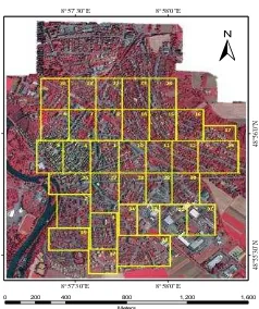
Both the true orthophoto (TOP) and the DSM are 9 cm ground sampling distance (GSD). For convenience, the large TOP and DSM are divided into 33 small tiles with different sizes according to the scene content, in total there are over 168 million pixels. At the same time, to evaluate the classification results of different methods and provide enough training samples for the supervised machine learning algorithm, manually labeled ground truth data for each tile are added to the dataset.
±
0 200 400 800 1,200 1,600 Meters
8°58'0"E 8°58'0"E
8°57'30"E 8°57'30"E
48
°5
6'
0"N
48
°5
5'
30
"N
±
Figure 2. The true orthophoto of the test area, which is divided into 33 tiles with different sizes.
3.2. Performance Analysis
For evaluating the proposed method deeply and objectively, in addition to the 16 tiles with publicly available ground truth, we also run our algorithm on the all 17 areas with undisclosed ground truth. we can see that most of buildings, trees and grass are labeled correctly, although there are some small objects and
pixels near the object boundary are misclassified. For assessing the results quantitatively, the accumulated confusion matrix and some derived measures (precision, recall and F1 score) for the whole unseen testing set are calculated and shown in Table 1. In (Mayer et al., 2006), Mayer et al. said in many cases if the classification correctness is around 85% and completeness around 70%, it can be used in real practical. By this criterion, our classification results can be considered relevant and useful for practical applications, except for the class “car”.
Table 2 shows the time costs at different stages of the proposed method for a tile with 2000x2500 pixels. From this we can see that at the stages of feature extraction and FCCRF refinement, the time costs are not too much. In contrast, most of time is spent on the RFE classification (1415s). Totally, the overall time for classifying the tile is about 25 minutes. We note that with the aid of high-performance GPU, Marmanis et al. (Marmanis et al., 2016) takes about 18 minutes (9 for coarse classification, another 9 for refinement) for classifying the same size tile with a state-of-the-art CNN-based method. Considering the fact that no GPU is used in our case, we think the proposed method is comparable to theirs in terms of computational efficiency.
ĘPredicted||
Reference ė Imp_surf Building Grass Tree Car Clutter
Imp_surf 91.9 2.9 3.6 1.0 0.8 0.0
Building 7.2 90.8 0.6 1.1 0.3 0.0
Grass 7.1 1.8 76.6 14.3 0.2 0.0
Tree 1.0 0.4 8.2 90.4 0.0 0.0
Car 37.1 7.4 0.8 0.4 54.3 0.0
Clutter 56.6 27.7 2.5 0.2 13.0 0.0
Precision/Correctness 84.9 93.9 84.2 85.1 54.4 -nan Recall/Completeness 91.9 90.8 76.6 90.4 54.3 0.0
F1 88.3 92.3 80.2 87.6 54.3 -nan
Overall accuracy 86.9
Table 1. Accumulated confusion matrix and some derived measures (precision, recall and F1 score) of ISPRS Semantic Labeling Contest benchmark on the unseen testing set.
Feature Extraction (s)
RFE
Classification (s)
FCCRF Refinement (s)
Time (s/tile) 108 1415 55
Table 2. Time costs at different stages of the proposed classification pipeline for a tile with 2000x2500 pixels
4. CONCLUSIONS
Our work brings together methods from RF and probabilistic graphical model for addressing the task of high-resolution remote sensing data classification. Starting from high resolution multi-spectral images and 3D geometry data, our method proceeds in three main stages: feature extraction, classification and refinement. 13 features (color, vegetation index and texture) from the multi-spectral image and 11 features (height, elevation texture and DMP) from the 3D geometry data are first extracted to form the feature space. Then the random forest is selected as the basic classifier for semantic classification. Inspired by the big training data and ensemble learning strategy adopted in machine learning and remote sensing community, a tile based scheme is used to train multiple RFs separately, and then combining them together to jointly predict each sample’s category probabilities. Finally the probabilities along with the feature importance indicator are used to construct a FCCRF graph model, and a mean-field
based statistical inference is carried out to refine the above classification results.
Experiments on ISPRS Semantic Labeling Contest data show that both features from the multi-spectral image and the 3D geometry data are important and indispensable for the accurate semantic classification, and multi-spectral image derived features play a greater role relatively. When comparing the classification accuracy of the single RF classifier and the fused RF ensemble, we found both the generalization capability and the discriminability are enhanced significantly. Consistent with the conclusions drawn by others, the smoothness effect of CRF is also evident in our work. Moreover, by introducing the top-3 most important features to the pairwise potential of CRF the classification accuracy is improved approximately by 1% in our experiments.
ACKNOWLEDGEMENTS (OPTIONAL)
This research was funded by: the Basic Research Fund of the Chinese Academy of Surveying and Mapping under Grant 777161103; (2) the General Program sponsored by the National
Natural Science Foundations of China (NSFC) under Grant 41371405.
REFERENCES
Marmanis, D., Wegner, J.D., Galliani, S., Schindler, K., Datcu, M., and Stilla, U., 2016. Semantic segmentation of aerial images with an ensemble of cnns. ISPRS Annals of the Photogrammetry, Remote Sensing and Spatial Information Sciences, III-3, pp.473-480.
Helmholz, P., Becker, C., Breitkopf, U., Büschenfeld, T., Busch, A., Braun, C., Grünreich, D., Müller, S., Ostermann, J., and Pahl, M., 2012. Semi-automatic quality control of topographic data sets. Photogrammetric Engineering & Remote Sensing, 78(9), pp.959-972.
Lu, Q., Huang, X., and Zhang, L., 2014. A novel clustering-based feature representation for the classification of hyperspectral imagery. Remote Sensing, 6(6), PP.5732-5753. Benediktsson, J.A., Palmason, J.A., and Sveinsson, J.R., 2005. Classification of hyperspectral data from urban areas based on extended morphological profiles. IEEE Transactions on Geoscience and Remote Sensing, 43(3), PP.480-491.
Shen, S., 2013. Accurate multiple view 3d reconstruction using patch-based stereo for large-scale scenes. IEEE transactions on image processing, 22(5), PP.1901-1914.
Furukawa, Y., and Ponce, J., 2010. Accurate, dense, and robust multiview stereopsis. IEEE transactions on pattern analysis and machine intelligence , 32(8), PP.1362-1376.
Vosselman, G., 2013. Point cloud segmentation for urban scene classification. ISPRS - International Archives of the Photogrammetry, Remote Sensing and Spatial Information Sciences, XL-7/W2(7), pp.257-262.
Zhang, J., Lin, X., and Ning, X., 2013. Svm-based classification of segmented airborne lidar point clouds in urban areas. Remote Sensing, 5(8), pp.3749-3775.
Zhang, J., and Lin, X., 2016. Advances in fusion of optical imagery and lidar point cloud applied to photogrammetry and remote sensing. International Journal of Image and Data Fusion, pp.1-31.
Rau, J.Y., Jhan, J.P., and Hsu, Y.C., 2015. Analysis of oblique aerial images for land cover and point cloud classification in an urban environment. IEEE Transactions on Geoscience and Remote Sensing, 53(3), pp.1304-1319.
Gerke, M., and Xiao, J., 2014. Fusion of airborne laserscanning point clouds and images for supervised and unsupervised scene classification. ISPRS Journal of Photogrammetry and Remote Sensing, 87(1), pp.78-92.
Khodadadzadeh, M., Li, J., Prasad, S., and Plaza, A., 2015. Fusion of hyperspectral and lidar remote sensing data using multiple feature learning. IEEE Journal of Selected Topics in Applied Earth Observations and Remote Sensing, 8(6), pp.1-13. Zhang, Q., Qin, R., Huang, X., Fang, Y., Liu, L., 2015. Classification of ultra-high resolution orthophotos combined with dsm using a dual morphological top hat profile. Remote Sensing, 7(12), pp.16422-16440.
Chen, L.C., Papandreou, G., Kokkinos, I., Murphy, K., and Yuille, A.L., 2016. Semantic image segmentation with deep convolutional nets and fully connected CRFs. Computer Science, (4), PP.357-361.
Gerke, M., 2015. Use of the stair vision library within the isprs 2d semantic labeling benchmark (vaihingen).
Paisitkriangkrai, S., Sherrah, J., Janney, P., and Hengel, A.V.D., 2015. In Effective semantic pixel labelling with convolutional networks and conditional random fields, IEEE Conference on Computer Vision and Pattern Recognition Workshops (CVPRW), pp.36-43.
Niemeyer, J., Rottensteiner, F., and Soergel, U., 2013. In Classification of urban lidar data using conditional random field and random forests, Urban Remote Sensing Event, pp.139-142.
Speldekamp, T., Fries, C., Gevaert, C., and Gerke, M. 2015. Automatic semantic labelling of urban areas using a rule-based approach and realized with mevislab, Technical Report, University of Twente.
Wei, Y., Yao, W., Wu, J., Schmitt, M., and Stilla, U., 2012. Adaboost-based feature relevance assessment in fusing lidar and image data for classification of trees and vehicles in urban scenes. ISPRS Annals of the Photogrammetry, Remote Sensing and Spatial Information Sciences, I (7), pp.138-139.
Krizhevsky, A., Sutskever, I., and Hinton, G.E., 2012. Imagenet classification with deep convolutional neural networks. Advances in Neural Information Processing Systems, 25, pp.1097-1105.
Sermanet, P., Eigen, D., Zhang, X., Mathieu, M., Fergus, R., and Lecun, Y., 2013. Overfeat: Integrated recognition, localization and detection using convolutional networks. Eprint Arxiv: 1312.6229.
Simonyan, K., and Zisserman, A., 2015. In Very deep convolutional networks for large-scale image recognition,
International Conference on Learning Representations (ICLR). He, K., Zhang, X., Ren, S., and Sun, J. 2015. Deep residual learning for image recognition, pp.770-778.
Sherrah, J. 2016. Fully convolutional networks for dense semantic labelling of high-resolution aerial imagery. Eprint Arxiv: 1606.02585.
Lin, G., Shen, C., Reid, I., and Hengel, A.V.D., 2016. Efficient piecewise training of deep structured models for semantic segmentation, IEEE Conference on Computer Vision and Pattern Recognition (CVPR), pp.3194-3203.
Long, J., Shelhamer, E., and Darrell, T., 2017. Fully convolutional networks for semantic segmentation, IEEE Transactions on Pattern Analysis and Machine Intelligence, 39(4), pp.640.
Papandreou, G., Chen, L.C., Murphy, K.P., and Yuille, A.L., 2015. Weakly-and semi-supervised learning of a deep convolutional network for semantic image segmentation, IEEE International Conference on Computer Vision (ICCV), pp.1742-1750.
Penatti, O.A.B., Nogueira, K., and Santos, J.A.D., 2015. Do deep features generalize from everyday objects to remote sensing and aerial scenes domains?, IEEE Conference on Computer Vision and Pattern Recognition Workshops (CVPRW), pp.44-51.
Ravinderreddy, R., Kavya, B., and Ramadevi, Y., 2014. A survey on svm classifiers for intrusion detection. International Journal of Computer Applications, 98(12), pp.34-44.
Hsu, C.W., Lin, C.J., 2002. A comparison of methods for multiclass support vector machines. IEEE transactions on Neural Networks, 13, pp.415-425.
Du, P., Xia, J., Zhang, W., Tan, K., Liu, Y., and Liu, S., 2012. Multiple classifier system for remote sensing image classification: A review. Sensors, 12(4), pp.4764-4792. Lu, D., and Weng, Q., 2007. A survey of image classification methods and techniques for improving classification performance. International Journal of Remote Sensing, 28(5), pp.823-870.
Briem, G.J., Benediktsson, J.A., and Sveinsson, J.R., 2002. Multiple classifiers applied to multisource remote sensing data.
IEEE Transactions on Geoscience and Remote Sensing, 40(10), pp.2291-2299.
Waske, B., and Benediktsson, J.A., 2007. Fusion of support vector machines for classification of multisensor data. IEEE Transactions on Geoscience and Remote Sensing, 45(12), pp.3858-3866.
Ceamanos, X., Waske, B., Benediktsson, J.A., Chanussot, J., Fauvel, M., and Sveinsson, J.R., 2010. A classiler ensemble based on fusion of support vector machines for classifying hyperspectral data. International Journal of Image and Data Fusion, 1(4), pp.1-15.
Pesaresi, M., and Benediktsson, J.A., 2001. A new approach for the morphological segmentation of high-resolution satellite imagery. IEEE Transactions on Geoscience and Remote Sensing , 39(2), PP.309-320.
Krähenbühl, P., and Koltun, V., 2013. Parameter Learning and convergent inference for dense random fields. International Conference on Machine Learning, 46, pp.346-350.
Mayer, H., Hinz, S., Bacher, U., and Baltsavias, E., 2006. A test of automatic road extraction approaches. International Archives of Photogrammetry, RemoteSensing and Spatial Information Systems, 36(3), pp.209-214.