A Modeling of Multi-
Echelon Suppliers’ Chain
for Deteriorating Items
Jonas Yu1,2, G.A. Widyadana3
Abstract: Inventory models for a policy of retail pricing and perishable items have been developed in many papers, but very few of the studies incorporate both of these effects. This study integrates the two conditions from a three-echelon supplier’s chain and offers a mathematical modeling for deteriorating inventory system with an optimal joint-cost policy. Exponentially deteriorating items with no shortages is assumed in this study. Two scenarios are considered. Scenario 1 assumed one supplier, one distributor and one retailer occurs at the regular inventory replenishment time, and scenario 2 assumes two suppliers, one distributor and two competitive retailers that to address this issue, we broaden the benchmark setting by letting the independent retailer channel be a duopoly. The mathematical model describes how the integrated approach to decision making can achieve global optimality as compared to independent decision by the suppliers, the distributor, and the retailers. A computer code is developed to derive the optimal solution. Numerical examples and sensitivity analysis are given to validate the results of the system.
Keywords: Deterioration, supply chain, three-echelon inventory system.
Introduction
Historically, the three key members of the supply chain, supplier, distributor and retailer, have been managed independently, buffered by large invento-ries. Increasing competitive pressures and decree-sing marginal profitability are forcing firms to develop supply chains that can quickly respond to customer needs and furthermore reduce the cost on carrying inventory. There are three fundamental stages in the supplier chain: Procurement, produc-tion and distribuproduc-tion. Through their coordinaproduc-tion, the number of deliveries is derived in corporation with each other to achieve a minimum overall inte-grated cost.
Deterioration is defined as decay, damage, spoilage, evaporation, obsolescence, pilferage, and loss of utility or loss of marginal value of a commodity that results in decreasing usefulness from the original one. Blood, fish, strawberries, alcohol, gasoline, radioactive chemicals and grain products are examples of deteriorating commodities. In this study, deterioration is assumed to be a function of the on-hand inventory within the whole supplier chain.
In order to reduce loss due to deterioration of the products, the members of the supply chains fre quently
1 Department of Information Management, Takming College, No.56, Sec.1, Huanshan Rd., Neihu District, Taipei 11451, Taiwan. Email: [email protected]
2 Institute of Industrial Management, National Central University, Chung-li 32054, Taiwan.
3 Faculty of Industrial Technology, Department of Industrial Engineering, Petra Christian University, JL. Siwalankerto 121-131 Surabaya 60238, Indonesia. Email: [email protected]
Invited Paper.
implement a joint decision to the optimal number of deliveries.
Ghare and Schrader [3] were the first authors to consider on-going deterioration of inventory. Then, several researchers have studied deteriorating inventory in recent decades. Bessler and Veinott [2] made the analysis on the integration between the buyer and the supplier by developing a mathematical model with an arborescent structure. Axsater [1] have developed the different models based on the centralized and decentralized echelon. Wee [7] derived the integration model between vendor and buyer for deteriorating items. Rau et al. [5] developed production inventory model for deteriorating items under multi echelon supply chain. Similar model is introduced by Rau et al. [6]. In their model they considered supplier-buyer integrated model by taking account buyer shoratage. Later Lin and Lin [4] developed two-echelon inventory model by considering completed backorder in the problem.
three-echelon inventory system usually happens in real life.
Methods
Mathematical Model
The mathematical model is developed on the basis of the following assumptions: (a) the demand rate is known and constant; (b) no shortage is allowed; (c) there is no constraint in space, capacity or capital; (d) the rate of replenishment in either distributor or retailers is infinite and on the same time; (e) a cons-tant fraction the on-hand inventory deteriorates and no replacement of deteriorated items is assumed; (f) only a single-product item is considered.
The following notation is used in this study:
: total joint cost for supply chain
: total cost for all retailers
: total cost for distributor
: total cost for all suppliers
: retailer’s inventory level at any time t,
: distributor’s inventory level at any time t
: suppliers’s inventory level at any time t, i = 1, 2
: ordering cost for retailers, : ordering cost for distributor : ordering cost for suppliers, i = 1, 2
: carrying cost per unit per unit time for retailers,
: carrying cost per unit per unit time for distributor
: carrying cost per unit per unit time for suppliers, i = 1, 2
: deterioration cost per unit per unit time for retailers,
: deterioration cost per unit per unit time for distributor
: deterioration cost per unit per unit time for suppliers, i = 1, 2
: demand rate for retailers,
: deterioration rate
: order arrangement rate, i = 1,2 : replenishment cycle time for suppliers : replenishment cycle time for retailers,i =
1,2,3….n
: replenishment cycle time for distributor : number of deliveries per cycle time T from
suppliers to distributor
: number of deliveries per cycle time tdfrom
distributor to retailers,
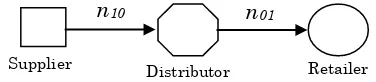
As an illustration, the supplier-distributor-retailer inventory system is depicted in Figure 1.
Figure 1. Supplier-distributor-retailer inventory system
We consider the supply chain system consisting of one supplier, one distributor and one retailer, purchasing an item through this chain.
The Retailers’ Deteriorating Inventory System
In general, a retailer’s deteriorating inventory system is described as follows:
Retail demand depends on two elements—primary demand for the product and store-level factors that
influence consumers’ sensitivity to retail.
Specifically, let p represent price, and retail demand be where >0represents the primary demand and >0 represents the store-level factors.
The consumers’ price decreases proportionally with
time going.
where represents the proportional number. The life cycle time of product is tl. It means the finished goods
should be sold out by the time.
The change inventory level, , during an infini-tesimal time, , is a function of the deterioration
rateα, demand rate d and the inventory level . It is formulated as
(1)
For a periodic cycle of , the inventory level and at the initial time, ; the solution of (1), after adjusting for the constant of integration is
[ ] (2)
From equation (1) and (2), the initial inventory level can be derived as:
(3)
and the deterioration amount during is
(4)
From equation (4), the carrying inventory during tri
can be derived as:
(5)
Supplier Distributor Retailer
Therefore, the retailer’s carrying cost for a periodic cycle is given by:
[ ] (6)
The retailers inventory cost per replenishment period trk is depicted by the following formula:
period cost = ordering cost + carrying cost + deteriorating cost
(7)
Thus, we obtain the total cost through the pro-duction cycle is given by:
∑ (8)
∑ ( )
where
(9)
The Distributor’s Deteriorating Inventory Sys-tem
The change inventory level, , during an infini-tesimal time, dt, is a function of the deterioration
rateα, demand rate dk and the inventory level .
It is formulated as
∑ (10)
For a periodic cycle of , the inventory level
and at the initial time, ; the solution of (11), after adjusting for the constant of integration is
∑ [ ] (11)
From equation (10) and (11), the initial inventory level can be derived as:
∑ ∑
( 12)
and the deterioration amount during td is
∑ ∑ (13)
Thus, the deterioration cost is
[ ∑ ∑ ∑
∑
] (14)
From equation (13), the carrying inventory during td
can be derived as:
[ ∑ ∑ ∑
∑
] (15)
Thus, the distributor’s carrying cost for a periodic cycle is given by:
(16)
Therefore, the total cost for distributor is
[ ∑ ∑ ∑ ∑
]
[ ∑ ∑ ∑
∑
] (17)
The Suppliers’ Deteriorating Inventory System
The change inventory level, , during an infinitesimal time, , is a function of the deterio-ration rate , demand rate , the order arrange-ment rate mi and the inventory level . It is
formulated as
∑ ,
where ∑ (18)
For a periodic cycle of T, the inventory level and at the initial time, ; the solution of (18), after adjusting for the constant of integration is
∑ [ ] (19)
From equation (18) and (19), the initial inventory level can be derived as:
∑ ∑
(20)
and the deterioration quantity during T is
(21)
Thus, the deterioration cost is
= ∑3=1
= ∑ +∑
3 =1 3
=1
∑3
=1
∑3 +
=1 ∑
+ � �
3
=1
The integrated total cost can be obtained as:
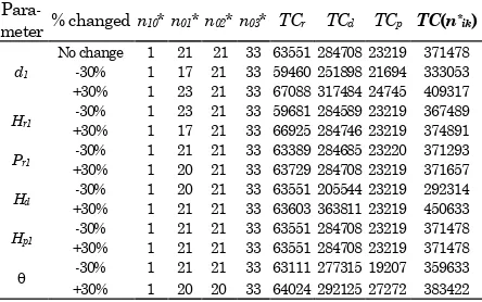
(26) sensitivity analysis for varying rates of demand, the
retailers’ carrying cost, the retailers’ deterioration cost, the distributor’s carrying cost, the suppliers’
carrying cost and rates of deterioration are tabulated in Table 2.
retailers’ carrying cost increases, the number of n*10 remains the same, but the number of n*01
tends to decrease. If the carrying cost decreases, the reverse is also true.
(3) As the retailers’ deterioration cost increases, the number of deliveries from distributor to retailers
tends to increase. Each player’s total cost, except the suppliers’ cost tends to increase. The joint
total cost TC increases as well.
(4) As soon as the deterioration rateαincreases, each
player’s total cost and the joint total cost tend to
increase. But, the number of deliveries remains the same.
(5) The joint total cost TC is more sensitive to the
parameter of the distributor’s carrying cost Hd. The
increase is over 20% as Hd increases by 30%.
Para-Conclusion
This paper discusses the optimal joint-cost policy in a two-suppliers three-echelon inventory model that integrates the upper, middle, and lower levels of the supply chain. By using the integrated approach that takes account of the suppliers, the distributor and the retailers, the total joint cost is found to be less than the independent approach by the individual player. The result is validated through sensitivity analysis. Furthermore, recent advances in communi-cations and information technology provide greater opportunity for significant savings in logistics cost by implementing strategic alliances within the supply chains.