www.elsevier.com / locate / econbase
New evidence on the effects of US monetary policy on
exchange rates
a b ,
*
Sarantis Kalyvitis , Alexander Michaelides
a
University of Cyprus and EMOP, Nicosia, Cyprus b
University of Cyprus, Department of Economics, P.O. Box 20537, Nicosia 1678, Cyprus
Received 19 May 2000; accepted 8 November 2000
Abstract
We examine the impact of US monetary policy shocks on exchange rates using the monetary policy indicator proposed by Bernanke and Mihov [Quarterly Journal of Economics, 113 (1998) 869–902]. We find evidence for instantaneous, rather than delayed, US dollar overshooting after a monetary shock when relative output and relative prices are included in the VAR specification. The forward premium puzzle persists due to the interest rate differential response. 2001 Elsevier Science B.V. All rights reserved.
Keywords: Monetary policy; Overshooting; Excess returns; Forward premium puzzle
JEL classification: E52; F31
1. Introduction
In a seminal paper Eichenbaum and Evans (1995) have shown that in response to tighter US `
monetary policy, the USDollar exhibits a ‘delayed overshooting’ pattern of 2 to 3 years vis-a-vis the major currencies (Japanese Yen, DMark, Italian Lira, French Franc, and Pound Sterling). ‘Delayed overshooting’ is confirmed by Evans (1994), who uses weekly data and finds that the USDollar
`
overshoots with a delay of 2 to 3 years vis-a-vis the DMark and the Yen, and Lewis (1995), who finds that the USDollar response relative to the DMark and the Yen increases for the first 5 months after the shock.
Eichenbaum and Evans (1995) also offer empirical evidence that after a contractionary US monetary shock, domestic interest rates rise as the USDollar appreciates. This creates a conditional
forward premium puzzle; by borrowing in Germany and investing in the US, for instance, positive
*Corresponding author. Tel.: 1357-2-892-109; fax: 1357-2-750-310.
E-mail address: [email protected] (A. Michaelides).
excess returns can be generated, conditional on tighter US monetary policy. Despite the fact that the ‘forward premium puzzle’ is well documented in empirical studies of the foreign exchange market, the puzzle now arises conditional on an exogenous change in US monetary policy.
These empirical findings are based on vector autoregressions (VARs) with US monetary policy
1
typically being identified by exogenous shocks in the Federal Funds rate or in non-borrowed reserves. In this paper, we re-examine the effects of US monetary shocks on the USDollar using an alternative measure of US monetary policy recently constructed by Bernanke and Mihov (1998). The Bernanke– Mihov (B-M) indicator has several advantages over previous approaches. Firstly, the specification is based on a model for commercial bank reserves and Federal Reserve operating procedures that nests most of the VAR-based indicators mentioned earlier. Secondly, the estimator is consistent with the estimated parameters describing the Fed’s operating procedure and the market for bank reserves. Thirdly, the indicator takes into account changes in the Federal Open Market Committee (FOMC) operating procedures and provides an optimal measure of monetary policy stance which may reflect both interest rate and reserves targeting.
In addition, we modify the original specifications by Eichenbaum and Evans (1995) to include relative output and relative prices as endogenous variables; this aims at capturing the relative business cycle position of the US and the foreign country, as well as long-run exchange rate adjustment based on Purchasing Power Parity. The recent strand of two-country open economy models suggests that the
relative position of the country is crucial for exchange rate determination (see, for instance, Obstfeld
and Rogoff (1996) for a textbook exposition). Interestingly, when relative output and prices are included in the VAR specification, the ‘delayed overshooting’ pattern disappears in most cases. On the other hand, excess returns continue to exist indicating that uncovered interest parity is still violated. The rest of the paper is structured as follows. Section 2 gives a brief account of the measurement and identification of US monetary policy shocks proposed by Bernanke and Mihov (1998) and outlines the methodology used in this paper. Section 3 discusses the empirical results from the VAR specifications and Section 4 concludes the paper.
2. Measures of US monetary policy and identification
To assess the effects of US monetary policy, a measure of such shocks is needed. There are two general categories of monetary policy measures. The first category is broadly known as the ‘narrative approach’ (Romer and Romer, 1989). Based on the minutes of the FOMC, these authors identify when policy-makers appeared to shift to a more anti-inflationary stance. The second general strategy for measuring monetary policy uses information about central bank operating procedures to develop data-based indexes of policy. In particular, data-based measures of monetary policy utilize restrictions imposed by central bank operating procedures to identify and estimate a VAR comprised of a set of macroeconomic and monetary policy variables.
1
Monetary policy shocks are identified as a disturbance term in the equation
Vt5z(Vt)1´t (1)
where V is the time t setting of monetary policy,t z is a (linear) function, Vt is the information
available to the monetary authority when policy is set at time t, and´t is a serially uncorrelated shock,
orthogonal to the elements of Vt. The measures arise from different specifications of Vt and V . Thet
shock ´t can reflect a number of random factors that affect policy decisions; these include the
personalities and views of the FOMC members, revisions of original data that cause members to change their opinion about the state of the economy, political and external factors, or other technical problems.
As is well known, for the period up to late 1979, and from 1983 onwards, the FOMC controlled closely the federal funds rate, allowing the quantity of reserves to vary. Instead, for the period starting from late 1979 to late 1982 the FOMC targeted directly non-borrowed reserves, with the federal funds rate moving freely (the Volcker disinflation period). This implies that for the period under investigation, the FOMC has exercised (at least) two types of monetary control. Any attempt to identify US monetary policy either by the federal funds rate or by changes in non-borrowed reserves
2
might result in a misspecified measure of the US monetary policy stance.
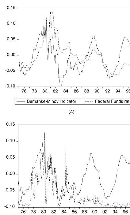
The B-M indicator explicitly addresses this potential misspecification by providing a measure of monetary policy which may reflect both interest rate and reserves targeting. Indeed, Bernanke and Mihov (1998) summarize their findings by arguing that ‘the Fed’s procedures appear to have changed over time, and hence no single model is optimal for the 1965–1996 time period. The FFR (federal funds rate) model is found to do well for the pre-1979 period, as argued by Bernanke and Blinder (1992), and it does exceptionally well for the Greenspan era, post-1988, which most Fed watchers would not find surprising. The FFR model also appears to be (marginally) the best choice for the sample period as a whole, based on both the monthly and biweekly results. As noted above, the NBR (non-borrowed reserves) model does well for the brief period of the Volcker experiment, 1979–1982, but is otherwise strongly rejected’. These results are graphically illustrated in Fig. 1A and B; the B-M indicator is very highly correlated with the federal funds rate except in the 1979–1982 period (Fig. 1A), when the indicator covaries positively with the ratio of non-borrowed to total reserves (Fig. 1B).
3. Empirical results for the USDollar with relative output and prices
To assess the impact of a monetary policy shock we estimate VARs of the following form:
k
Zt5A01
O
A Z1 t2i1ut (2)i51
2
Fig. 1. (A) Bernanke and Mihov (1998) US monetary policy indicator and the Federal Funds rate; (B) Bernanke and Mihov (1998) US monetary policy indicator and the non-borrowed to total reserves ratio.
where A is an n0 31 vector of constants, A are n1 3n matrices of coefficients and u is an nt 31
9
9
vector of residuals with E(u )50, E(u u )50;t±s, E(u u )5S;t5s and S defined as a
t t s t s
symmetric positive semidefinite matrix. The results were generated with monthly data covering the period 1975:01 to 1996:12 (the B-M indicator is available until 1996:12; see Appendix A for a more detailed description of data sources). All VARs in this section were estimated, after testing the robustness of the results to higher order specifications, with a 6-month lag length.
After dropping time subscripts for simplicity, our five-variable VAR consists ofhIPUS / For, PUS / For,
US / For
B-M, (RFor2RUS), st j, where IPUS / For is the log of industrial production in the US to the foreign
country, PUS / For is the log of the price level in the US to the foreign price level, B-M is the indicator
of monetary policy, (RFor2RUS) denotes the difference between short term interest rates, where RFor
US / For
and RUS denote the foreign and US short term interest rates, respectively, and st denotes the log
3
of the nominal exchange rate with respect to hYen, DMark, Lira, Franc and Sterlingj, at time t. The
quantitative characterization of the exchange rate response to a monetary policy shock is provided by impulse response functions. Consider, in particular, the effect of a monetary shock at time t on the
exchange rate between months t1i and t1j with j.i. In population, these responses are equal to
4
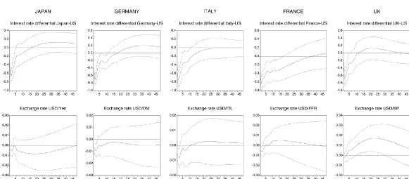
the average value of the coefficients i through j of the corresponding impulse response functions. Fig. 2 displays the dynamic response functions of the interest rate differential and the USDollar exchange rate to a contractionary US monetary policy shock as illustrated by a standard deviation shock to the B-M indicator. Dotted lines denote standard errors of impulse responses at the 95% confidence level derived over 500 Monte Carlo draws from the estimated asymptotic distribution of the VAR coefficients and covariance matrix of the innovations.
Interest rate differentials are diminished after the shock and remain lower and statistically different
from zero for |6 months in Japan and the UK, 11 months in Germany and Italy and 17 months in
France. On the other hand, there is a statistically significant appreciation of the USDollar for around 3 months after the shock for all the currencies involved; note, however, that the appreciation is instantaneous rather than displaying ‘delayed overshooting’. The only difference occurs in the case of
Sterling, which depreciates against the USDollar |1 year after the shock and remains statistically
different from zero for around 2.5 years after the initial shock.
5
How do relative prices and relative output respond to a tighter US monetary stance? The rise of `
the US interest rate differential vis-a-vis the rest of the countries triggers a decline in relative output.
The fall is significant in the cases of Japan, Germany and France, lasting up to |3 years. The effect on
relative prices is not statistically significant, however.
Even though ‘delayed overshooting’ does not arise in the current set-up, uncovered interest parity is still violated. Responses are generated by the model after replacing the interest rates and the real exchange rate with excess returns, defined as
US / For US / For US / For
xr 5RFor2RUS1st11 2st . (3)
6
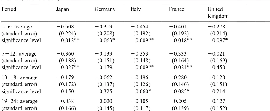
Ex post excess returns exist for all countries (see Table 1), but in the cases of UK and Germany these are significant at the 10% level only for the 6-month period following the shock. On the other
3
Using the real, rather than the nominal, exchange rate leads to nearly identical conclusions about the response of the exchange rate to the monetary policy shock. This result arises because nominal and real exchange rates are highly correlated at the monthly frequency for the countries under consideration.
4
Note that previous studies that have used data based indices of monetary policy have been criticized on the grounds of the ‘price puzzle’; US prices are predicted to rise in estimated VARs in response to tighter US monetary policy. Sims (1992) argues that the result can be attributed to the fact that the Fed takes into account commodity price inflation in its reaction function, while this variable was omitted from previous VARs. We did not include the commodity price index in our set of variables, because the B-M indicator controls explicitly for the effect of commodity prices on US monetary policy.
5
The results are not reported here; these are available from the authors upon request. 6
S
.
Kalyvitis
,
A
.
Michaelides
/
Economics
Letters
71
(2001
)
255
–
263
Table 1
Dynamic responses of excess returns: model: hUS foreign industrial production, US foreign prices, Bernanke–Mihov a
indicator, excess returnsj
Period Japan Germany Italy France United
Kingdom
1–6: average 20.508 20.319 20.454 20.401 20.278 (standard error) (0.224) (0.208) (0.192) (0.192) (0.214) significance level 0.012** 0.063* 0.009** 0.018** 0.097*
7212: average 20.360 20.139 20.353 20.333 20.021 (standard error) (0.188) (0.151) (0.148) (0.164) (0.169) significance level 0.027** 0.179 0.009** 0.021** 0.450
13–18: average 20.179 20.062 20.196 20.280 20.120 (standard error) (0.172) (0.137) (0.126) (0.146) (0.151) significance level 0.150 0.325 0.060* 0.085* 0.214
19–24: average 20.038 0.020 20.105 20.205 0.127 (standard error) (0.166) (0.145) (0.117) (0.139) (0.152)
significance level 0.409 0.445 0.186 0.070* 0.203
a
Excess returns are monthly earnings from investing in the foreign country relative to an investment in the US. See also Eichenbaum and Evans (1995).
An asterisk denotes significance at the 10% level and two asterisks at the 5% level.
hand, returns are significant in the case of Japan for a year after the shock, Italy (for 18 months following the shock), and France (for 2 years following the shock). Given the exchange rate response, these excess returns can be accounted for by the persistent widening of the interest rate differential in favor of the US.
4. Conclusions
This paper has re-investigated the effects of US monetary policy shocks on the USDollar. Building on the work of Eichenbaum and Evans (1995), we provide further evidence on the effects of US monetary policy on exchange rates. These authors have shown that a US monetary contraction generates a persistent appreciation of the USDollar (‘delayed overshooting’) combined with a persistent widening of the US–foreign interest rate differential, which generates a conditional forward premium puzzle.
countries under consideration due to the widening of the US–foreign interest rate differential stemming from the contractionary shock in US monetary policy.
Acknowledgements
We would like to thank Ben Bernanke and Ilian Mihov for kindly providing us with the indicator of US monetary policy and Ben Bernanke, Ilian Mihov and Nikitas Pittis for helpful comments and suggestions. The first author acknowledges financial support from TMR Project ERBFMRXCT98-0213 and the second from a University of Cyprus research grant. All remaining errors or omissions are our own.
Appendix A. Data
The data used in the study were extracted from the following sources.
Nominal exchange rates: all exchange rates are from the IFS CD ROM and are bilateral monthly
exchange rates constructed using the following IFS foreign currency per USDollar exchange rates: 158..AF.. is the Japanese Yen, 134..AF.. is the DMark, 136..AF.. is the Italian Lira, 132..AF.. is the French Franc, and 112..AF.. is British Sterling.
Short term interest rates: the interest rates are from the IFS CD ROM: 15860B.. for Japan (call
money), 13460B.. for Germany (call money), 13660B.. for Italy (money market), 13260B.. for France (call money), 11260B.. for UK (overnight interbank). For the US 11160B.. is the federal funds rate FYFF.
Industrial production: for all countries industrial production (seasonally adjusted) is from the
OECD database.
Price level: the data are collected from the OECD, CITIBASE and IFS databases; for all countries
the Consumer Price Index was used, except for the UK where the Retail Price Index (all items) was used.
References
Bernanke, B., Blinder, A., 1992. The Federal Funds rate and the channels of monetary policy transmission. American Economic Review 82, 901–921.
Bernanke, B., Mihov, I., 1998. Measuring monetary policy. Quarterly Journal of Economics 113, 869–902.
Bonser-Neal, C., Roley, V., Sellon, G. Jr., 1998. Monetary policy actions, intervention and exchange rates: a reexamination of the empirical relationships using federal funds rate target data. Journal of Business 71, 147–177.
Christiano, L., Eichenbaum, M., Evans, C., 1999. Monetary policy shocks: what have we learned and to what end. In: Taylor, J., Woodford, M. (Eds.). Handbook of Macroeconomics, Vol. 1A. North-Holland, Amsterdam, pp. 65–148. Dornbusch, R., 1976. Expectations and exchange rate dynamics. Journal of Political Economy 84, 1161–1176.
Eichenbaum, M., Evans, C., 1995. Some empirical evidence on the effects of shocks to monetary policy on exchange rates. Quarterly Journal of Economics 110, 975–1009.
Evans, C., 1994. Interest rate shocks and the dollar. Economic Perspectives, Federal Reserve Bank of Chicago 18, 11–24. Lewis, K., 1995. Are foreign exchange intervention and monetary policy related, and does it really matter? Journal of
Obstfeld, M., Rogoff, K., 1996. Foundations of International Macroeconomics. MIT Press, Cambridge.
Romer, C., Romer, D., 1989. Does monetary policy matter? A new test in the spirit of Friedman and Schwartz. In: Blanchard, O., Fischer, S. (Eds.), NBER Macroeconomics Annual. MIT Press, Cambridge.
Sims, C., 1992. Interpreting the macroeconomic time series facts: the effects of monetary policy. European Economic Review 36, 975–1000.