CROP TYPE MAPPING FROM A SEQUENCE OF TERRASAR-X IMAGES WITH
DYNAMIC CONDITIONAL RANDOM FIELDS
B. K. Kenduiywoa∗, D. Bargiela, U. Soergelb a
Institute of Geodesy, Technische Universit¨at Darmstadt, Germany - (kenduiywo, bargiel)@geod.tu-darmstadt.de bInstitute for Photogrammetry, University of Stuttgart, Germany - [email protected]
Commission VII, WG VII/4
KEY WORDS:Dynamic Conditional Random Fields (DCRFs), conditional random fields (CRFs), phenology, spatial-temporal clas-sification, TerraSAR-X
ABSTRACT:
Crop phenology is dynamic as it changes with times of the year. Such biophysical processes also look spectrally different to remote sensing satellites. Some crops may depict similar spectral properties if their phenology coincide, but differ later when their phenology diverge. Thus, conventional approaches that select only images from phenological stages where crops are distinguishable for classifica-tion, have low discrimination. In contrast, stacking images within a cropping season limits discrimination to a single feature space that can suffer from overlapping classes. Since crop backscatter varies with time, it can aid discrimination. Therefore, our main objective is to develop a crop sequence classification method using multitemporal TerraSAR-X images. We adopt first order markov assumption in undirected temporal graph sequence. This property is exploited to implement Dynamic Conditional Random Fields (DCRFs). Our DCRFs model has a repeated structure of temporally connected Conditional Random Fields (CRFs). Each node in the sequence is connected to its predecessor via conditional probability matrix. The matrix is computed using posterior class probabilities from asso-ciation potential. This way, there is a mutual temporal exchange of phenological information observed in TerraSAR-X images. When compared to independent epoch classification, the designed DCRF model improved crop discrimination at each epoch in the sequence. However, government, insurers, agricultural market traders and other stakeholders are interested in the quantity of a certain crop in a season. Therefore, we further develop a DCRF ensemble classifier. The ensemble produces an optimal crop map by maximizing over posterior class probabilities selected from the sequence based on maximum F1-score and weighted by correctness. Our ensemble technique is compared to standard approach of stacking all images as bands for classification using Maximum Likelihood Classifier (MLC) and standard CRFs. It outperforms MLC and CRFs by 7.70% and 6.42% in overall accuracy, respectively.
1. INTRODUCTION
Food security is a matter of concern globally. Shortage of food can lead to socio-economic consequences. Foresight by the world bank estimates that since 2010 demand for food has in-creased resulting into extreme poverty of about 44 million peo-ple (World-Bank, 2011). Estimated rise in population and diets will require significant increase in food production (Tilman et al., 2011). Therefore, current efforts by farmers, agronomist and re-lated stakeholders is to ensure that food production is optimal and sustainable. This demands regular update of spatial and tem-poral information on agriculture activities to aid monitoring and sustainable food policy decision making. Such information is to be derived from a dynamic phenomenon over a vast area. Thus, methods of data collection that can match this scale are necessary.
Remote sensing satellites capture spectral, spatial and temporal attributes of phenomena on the earth surface. This is because of their specific electromagnetic spectrum sensitivity, synoptic view and temporal capability. Mapping agriculture activities requires insights on crop dynamics, e.g. phenology1 states and seasonal growth. Spectral trend of agricultural parcels is constantly chang-ing. Different crops may at a given time be in the same pheno-logical state, depicting similar spectral attributes, but differ sig-nificantly in another time (Siachalou et al., 2015). According to Siachalou et al. (2015), crop mapping using single-date remote sensing images, even if acquired in critical growth stages, can not
∗Corresponding author.
1In remote sensing we can consider phenology as the appearance of a
crop at a particular instance in its life cycle.
offer optimal results in case of crops with similar phenology. A sequence of multitemporal images and phenological information can be integrated using a robust statistical framework to improve crop discrimination.
This study adopts a sequence of Synthetic Aperture Radar (SAR) images from TerraSAR-X satellite for crop classification. Radar satellites are daylight and weather independent. Signals from radar can penetrate vegetation canopy and dry soil thus bearing volumetric and subsurface information. These attributes renders SAR a good medium to deliver a sequence of images of high-est temporal density suitable for crop classification regardless of climatic zones. In contrast, complexity, e.g. speckle inter-ference, accompanying SAR data challenges conventional pixel based approaches. Spatial context can be employed to over-come it (Kenduiywo et al., 2014). However, crops in the same phenology exhibit correlated SAR backscatter. Conventional approaches stack multitemporal images as bands for classifica-tion (e.g., Bargiel and Herrmann (2011); Forkuor et al. (2014); Sonobe et al. (2014)). By doing so, significant temporal informa-tion from satellite observed crop phenology is limited to a sin-gle feature space. Discrimination in such feature space can suf-fer from overlapping class boundaries due to large class variance from spectral variation. In addition to spatial context, integra-tion of temporal context in a principled manner can help resolve classes over time.
classification adopting spatial context also exist (Ozdarici-Ok et al., 2015; Roscher et al., 2010). Efforts to use both spatial and temporal context to classify crops from optical images is done in (Hoberg and M¨uller, 2011). The study models temporal con-text via a global transition matrix determined from training data. A global matrix assumes similar phenology transitions over all pixels neglecting changes that may exist in the image. In our previous study (Kenduiywo et al., 2015), pixel-wise temporal in-formation exchange between grouped crop classes in two epochs2 are considered. Here, the approach is extended to a dynamic tem-plate that classifies each crop type over a sequence of multitem-poral SAR images.
The contributions of this study are threefold: (1) to develop a spatial-temporal classification framework to discriminate crops using a sequence of multitemporal TerraSAR-X images, (2) de-sign a suitable spatial interaction model, modified from contrast sensitive model suggested by Shotton et al. (2009), to moderate changes in class labels based on data evidence and (3) to design an ensemble framework to generate an optimal season crop map. We used dynamic conditional random field(s) (DCRFs) for se-quence crop classification. The framework allows reasoning via Bayesian theory in a principled statistical manner under uncer-tainty. We incorporate DCRF into standard conditional random fields (CRFs) as a temporal classifier template. This forms a ro-bust spatial-temporal sequence crop classifier termed as DCRF because: (a) of a changing probabilistic relational model between nodes in the sequence, (b) the model captures time-changing phe-nomena, encodes complex interactions over the set of all possi-ble classes and data and uncertainty in a principled manner, and (c) the model is a conditional distribution that factorizes accord-ing to an undirected graphical model whose structure and param-eters are repeated over a sequence (Sutton et al., 2007).
The rest of the paper is organized as follows. Section 2 intro-duces the approach we adopted and illustrates how CRF is de-signed for spatial-temporal crop sequence classification. Section 3 describes selected study area, crops considered for classifica-tion, data and features used, details of experiments conducted by our design and other methods. In Section 4, a description of re-sults from our technique compared to others is made leading to a discussion in Section 5. Conclusions from the study and future tasks are provided in Section 6.
2. METHODS
2.1 Conditional Random Fields
Conditional Random Fields were introduced by Lafferty et al. (2001) for one-dimensional text classification and extended to two-dimensional image classification (Kumar, 2006). They are undirected graphs which represent conditional probability distri-bution over a set of data/data sequence. The conditional probabil-ities are represented in non-negative functions, potentials, defined over a subset of fully connected variables known as cliques3. In CRFs, posterior probability of a distribution is computed as a product of potentials through inference techniques.
DefinitionConsider a sequence of imagesx=xtmodelled over
corresponding discrete labelsy= yt, from a given set of class
labelsl ∈m, acquired at different timestwheret= 1, . . . , T. LetG={S, E}be a graph with spatial edgesEdefined over a pair of cliquesiandjin a neighbourhood setN such thaty= (yi)i∈Swhereyis indexed by nodes (vertices)Sof the Graph
2An epoch is an image date within a sequence of acquired images. 3A clique is a fully connected subgraph.
G. In mono-temporal classification, the random variable (y, x) is a CRF only if, when conditioned onx, the random variable
yiobeys the Markov property with respect to G:P(yi|x,y\i) = P(yi|x,yNi), wherey\i is the set of all nodes in the G except
nodeiandNiis a set of neighbours of nodeiin G.
Following Hammersley and Clifford basic theorem, the joint dis-tribution over the labelsygiven the dataxcan be written as:
P(y|x) = 1
where Z(x) is a normalizing constant referred to as partition function, andAandIare the association (unary) and interaction (pairwise) potentials respectively.
2.2 Dynamic conditional random fields
Sequence classification requires determination of posterior prob-abilityP(y1,...,T|x1,...,T). The computation is intractable and
ex-ponential in time as it involves estimation ofSTfunctions in a
2-D space. Since satellite observation of crops is unique in each in-stance, we assume that their evolution is independent. In this way, the conventional class conditional independence (Swain, 1978) can be attained:P(y1,...,T|x1,...,T) =P(y1|x1), . . . , P(yT|xT).
This simplifies the classification problem to an independent esti-mation of class posterior probabilitiesP(yi)for each nodeiin t. Spatial interactions are also considered at each epoch byIin Eq. (1).
To exploit crop phenological information, we extend DCRFs pro-posed by Sutton et al. (2007) for text sequence classification to 3-D image sequence classification. A DCRF is a conditionally-trained undirected graphical model whose structure and parame-ters are repeated over a sequence. We developed an undirected DCRF graph template that factorizes according to first order Markov assumption. In the design, each node iat timetcan depend on node data from the previous (ift6= 0) and subsequent (ift6=T) epochs. The objective is to connect a set of all possi-ble temporal cliquesCof nodesSusing a conditional probability matrix distributionP(y|yt−1,x,xt−1). This set-up gives a DCRF sequence template model, considering crop phenology, such that a node can have at least one or two temporal neighbours (Fig. 1).
DefinitionLetc,c∈ C, be a temporal clique index of a nodek
in epoch∆t=t−1of a label vectory∆twhich corresponds to
another nodeiin label vectorytat timetsuch thatc={k,∆t}. In this case, a set of random variablesyi,t,c≡ {yi,t|(k,∆t)∈c}
is the set of variables of the evolving clique indexcat timetin the sequenceT. Then, our spatial-temporal DCRF template can be expressed as:
whereT P is temporal potential.
2.2.1 Association Potential determines how likely an image siteitakes a labelyigiven the datax:A(yi,x) =P(yi|fi(x)),
fi(x)is a site-wise feature vector (Kumar, 2006). We used
t = 1
t = 2
t = 3
t = T
Figure 1. First order temporal neighbours of a node at different timestof a sequenceT. Spatial and temporal edges are
indicated by solid and dashed lines respectively.
are unique over the sequence. A RF conducts classification by casting votes from a number of decision treesDTgenerated
dur-ing traindur-ing. If the number of votes cast for a given class labely
by RF isVy, then ourAat siteiisP(yi =y|fi(x)) = We setDT = 250because over 200 trees RF stabilizes (Hastie
et al., 2011) and set tree depth as 25.
2.2.2 Interaction Potential measures the influence of data and neighbouring labels on sitei. It ensures that sitei, as ini-tially determined by association potential, is labelled to its corre-sponding ”true class” given data evidencexand neighbourhood dependencyN wherej ∈ Ni. We setN = 8, second order
neighbourhood structure, as shown in Fig. 1. This study modelled
Iby comparing two models: contrast sensitive model suggested in (Shotton et al., 2009),
I(yi, yj,x) =
(
β·exp (−η·dij) ifyi=yj
0 ifyi6=yj
(3)
and a new version of contrast sensitive Potts model:
I(yi, yj,x) =
(
β·exp (−η·dij) ifyi=yj
β·(M ax[1−exp(−η·dij), ǫ])−1 ifyi6=yj
(4)
whereβis a spatial interaction parameter that regulates smooth-ness, parameterηweights and controls inclusion (η >0) or
ex-clusion (η = 0) of data interactionsdij =
√PR
i=1|fi(x)−fj(x)|2
R
of adjacent node features fi and fj, R is the number of
fea-tures/elements in vectorsfiandfj,M axis a function that returns
a maximum between two values andǫis a value close to zero (it prevents division by zero). Since data interactions are considered in CRF, by defaultη >0. Division byRensures identical influ-ence ofIover the sequence of imagesT. Therefore, the model is different from contrast sensitive Potts model because transitions of adjacent labels are now moderated based on data evidence both when initial labels fromAare similar or dissimilar. In this
man-ner, the model regulates smoothing while preserving edges.
2.2.3 Temporal Potential models interactions between nodes in the sequence of imagesT. This potential can be considered as a classifier that ensures mutual information exchange between nodesiandkin epochtand∆t. Since the posterior probabilities
P(yi =l)andP(yk=l)are determined byA, ourT P can be
expressed as:
T P(yi,t,c,x,x∆t) =P(yi=l|yk=l) (5)
To solve Eq. (5), Bayesian formula is used to compute conditional probability matrix ofT Pas:
P(yi=l|yk=l) =
P(yi=l, yk=l)
P
yiP(yi=l, yk=l)
(6)
Eq. (6) determines the probability of a crop labell ∈ mbeing assigned to a nodeigiven data from the two epochstand∆t. It is used to compute a pixel-wise conditional probability matrix as shown in (Kenduiywo et al., 2015).
2.3 Optimal crop mapping with DCRF
In most cases farmers, governments, and other stakeholders are interested in the quantity of a certain crop in a given season. Our DCRF approach incorporates phenological information exchange between each epoch given a preceding one and vice versa. At each epoch we obtain posterior class probabilities incorporating phenological information in images. For this reason, we develop an ensemble classifier to generate an optimal seasonal crop map.
Consider our classification problem where each nodei∈Sis to be assigned a discrete class labelyfroml∈mpossible classes (y1, . . . , ym) in each epochtfrom the sequenceT. Now given
that posterior probabilitiesP(yl|x, t)have been determined, then
for each classlwe select a probability with maximum F1-score from the sequenceTand weight them with correctness accuracy. Then, a discrete class for nodeican be determined by maxi-mizing over probabilities selected from the sequence. Since the same training sites are used throughout the sequence (crop sea-son), then prior probability are assumed equal:
ˆ
with maximum F1-score (Sokolova et al., 2006), i.e. F1 =
2(correctness×completeness)
correctness+completeness , at timet, Corris the correctness
accuracy measure andyˆithe estimated class label. Correctness
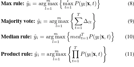
and completeness correspond to recall and precision respectively. This approach, Eq. (7), is compared to the following classifier combinations rules in (Kittler et al., 1998):
Max rule:yˆi=
A Posterior (MAP) estimate. This requires an inference algorithm to determine posterior probabilitiesP(y|x)and a maximization algorithm to estimate optimum labelsyˆ. We apply sum-product Loopy Belief Propagation (LBP) (Murphy et al., 1999), a stan-dard inference algorithm in graphs with cycles. To estimate class labels, we design a maximization algorithm. The association po-tential probabilities used in bothIandT P are trained using RF implemented in OpenCV (OpenCV, 2014).
3. EXPERIMENTS
3.1 Study area and data
The study area is located in Northern Germany (52.26◦N,
9.84◦E), see Fig. 2. The average annual precipitation and tem-perature are 656 mm and8.9◦C respectively (Deutscher Wetter-dienst, 2012). The region is characterized by intensive agriculture with large farms. Crops in the area include: 1) barley, 2) canola, 3) grassland, 4) maize, 5) oat, 6) potato, 7) rye 8) sugar beet and, 9) wheat. These crops go through different phenological stages within a season, a fact that can enhance discrimination. Four phenology phases, preparation, seeding, growing, harvest-ing and post harvest, are considered (Fig. 3). Preparation phase involves ploughing and soil grooming processes before seeding. In seeding phase, crop seeds are placed in the soil. Growing phase includes the period between crop germination to ripening. After ripening, harvesting starts by gathering mature crops from the fields. The last stage is post harvest phase, where the field could be fallow or with some remaining ripe crops.
´
0 450 Km
Legend
study site agricultural areas
non agricultural areas
´
0 1 2 3 4
Kilometers
´
Figure 2. Study area.
Jan Feb Mar Apr May Jun Jul Aug Sep Oct Nov Dec
Maize
Potato
Canola
Sugar beet
Oat
Barley
Wheat
Rye
Grassland
Jan Feb Mar Apr May Jun Jul Aug Sep Oct Nov Dec
Preparation Seeding Growing Harvesting Post Harvest
Figure 3. Phenology stages of crops considered for classification.
The temporal sequence consists of six dual polarized (HH and VV) TerraSAR-X High Resolution Spotlight images acquired on:
11thMarch, 13thApril,22ndMay, 18thJune,10th June and
17thOctober in the year 2009. All are acquired at an incidence
of34.75◦with range and azimuth resolutions of 2.1 m and 2.4 m except for the month of May which has an incidence angle of
43.65◦with range and azimuth resolutions of 3.4 m and 2.9 m. The images were delivered as ground range products (MGD) with equidistant pixel spacing. They are radiometrically calibrated to
σ0 according to Fritz and Eineder (2009). All images are co-registered to an extent of 7.1×11.8km2 using WGS 1984 da-tum on UTM Zone 32N coordinate projection system. Our ex-periment site covers an extent of 5.4×5.4km2.
Reference data campaign was conducted concurrently with image acquisition during the year. The reference parcels were separated into training and validation sets using stratified random sampling design tool in ArcGIS 10.0 (Buja and Menza, 2013). Distribu-tion of each crop type (training set / validaDistribu-tion set) in hectares is: barley (38.54 / 41.30), canola (38.60 / 40.87), grassland (69.97 / 55.10), maize (27.63 / 33.10), oat (10.11 / 17.39), potato (55.76 / 66.45), rye (97.23 / 79.04), sugar beet (52.49 / 47.51), and wheat (34.88 / 34.84).
3.2 Feature selection
Gray Level Co-occurence Measures (GLCM) were computed us-ing a3×3matrix. Eight features — mean, variance, correlation, homogeneity, contrast, dissimilarity, entropy and 2nd moment — were computed in directions0◦,45◦,90◦, and135◦giving rise to a total of 32 features in each polarization. Random Forest vari-ance importvari-ance was used to select 4 significant features from the 8 GLCM features in each direction and polarization (a total of 32 features per epoch). Important GLCM features as per RF include: correlation, homogeneity, variance and mean. For each selected feature, a super pixel/block was generated from a mean of3×3pixels. Block size selection was done in consideration to the minimum mappable unit. The shift from pixels to block seg-ments classification is advocated in (Blaschke and Strobl, 2001).
3.3 Parameter determination
Selection of a model forIand its parameters is an important step in CRF classification. Thus, we conducted classification tests us-ing models in Eqs. (2) and (3) over a range ofβandη param-eter values in 2-D logarithmic scale. Epochs in growing season (June and July) are adopted to compute average overall classifi-cation accuracy for each set of parameters. These epochs were chosen because within the period, returned radar backscatter are dominantly from crops. A suitable model ofIincludingβandη
parameters are then selected using initial 2-D logarithmic scale search results.
3.4 Classification
We adopt the technique in Eq. (2) for crop sequence classifica-tion. The approach classifies each epoch integrating first order temporal information and spatial information from 8 neighbour-ing nodes. We compare this approach to MLC, RF (association potential) and mono-temporal CRF (CRF-mono), Eq. (1), in sin-gle epoch classification.
4. RESULTS
4.1 Feature selection results
Results of GLCM features selection are described here. Four fea-tures were selected using RF variable importance criteria. Fig. 4 shows RF importance computed from an average of four di-rections, 0◦, 45◦, 90◦, and135◦, for each feature and subse-quently their average over epochs. Generally with the exception of HH-polarized correlation features, features computed from VV-polarization backscatter have a higher importance compared to features computed from HH-polarization.
0.00 0.01 0.02 0.03 0.04 0.05 0.06 0.07 0.08 0.09
V
a
ri
a
bl
e
I
m
po
rt
a
n
c
e
VV
HH
Figure 4. Average random forest variable importance for different GLCM features.
4.2 Parameter determination results
Selection of a data interaction model forI and its correspond-ing parameters was guided by results in Fig. 5. The new ex-panded contrast sensitive model, Eq. (4), outperforms standard contrast sensitive, Eq. (3), in overall accuracy (OA) with most parameters. Our new model gives high classification accuracy for101 ≤beta≤103and10−2 ≤eta≤5. In contrast, accu-racy for contrast sensitive Potts model reduces ifbeta >0.1in combination with anyetaparameter values. This search, with a compromise between high accuracy and over-smoothing, guided our choice ofβ= 10andeta= 1for our new data dependent in-teraction model in Eq. (4). We use these parameter values across the sequence for comparability.
4.3 Classification results
Results from DCRF epoch classification compared to other ap-proaches are illustrated in Fig. 6. The results show that DCRF approach outperforms CRF-mono, RF and MLC. In all epochs MLC has the least accuracy followed by RF and CRF-mono re-spectively. The addition of temporal information also improved classification accuracy in each epoch since DCRF outperformed CRF-mono which considers only spatial information. Spatial in-formation also improved classification as demonstrated by CRF-mono performance compared to RF and MLC which have lower accuracy.
An optimal crop map is generated from epoch-wise DCRF poste-rior probabilities using different classifier combination strategies as depicted by results in Table 1. The technique we introduce, DCRF max F1-score, outperforms max rule, majority vote, prod-uct rule and median rule by 33.92%, 10.04%, 7.91% and 7.85% in
η
β
10−2 10−1 100 101 102 10−2
10−1 100 101 102
103
37 42 51 53
OA (%)
(a)
η
β
10−2 10−1 100 101 102 10−2
10−1 100 101 102
103
36 37 42 43
OA (%)
(b)
Figure 5. Comparison of our new spatial interaction model Fig. 5a and contrast Potts model Fig. 5b over a logarithmic scale.
0% 10% 20% 30% 40% 50% 60% 70%
March April May June July October
DCRF OA CRF OA RF OA MLC OA
DCRF Kappa CRF Kappa RF Kappa MLC Kappa
Figure 6. Epoch-wise classification results, overall accuracy and kappa, from different approaches.
overall accuracy respectively. Thus, max rule has the least overall accuracy followed by majority vote, median rule and product rule respectively.
Method OA Kappa
Max Rule 40.61% 33.59%
Majority Vote 64.49% 59.41% Median Rule 66.68% 61.80% Product Rule 66.62% 61.71% Max F1-Score 74.53% 70.98%
Table 1. Comparison of different strategies of integrating DCRF posterior probabilities to produce an optimal classification map.
clas-sifiers as opposed to a limited view on overall accuracy in Ta-ble 2. It is only grassland that has a lower classification accuracy in our approach (correctness -16.4% / completeness -2.3%) com-pared to MLC-stack approach. All other classes were classified better or comparable to MLC-stack approach. This is especially true for barley (+17.05% / +2.01%), maize (+24.33% / +18.58%), oat (+19.99% / +13.45%) and sugar beet (+45.83% / +21.93%). Rye and wheat also slightly improved (+5.58% / +2.03%) and (+5.65% / +5.80%) respectively, while canola and potato exhibit a lower correctness of -5.88% and -3.40% but a higher complete-ness of +2.70% and +10.70%.
Method OA Kappa
MLC-stack 66.83% 61.67%
CRF-stack 68.11% 63.33%
DCRF max F1-Score 74.53% 70.98%
Table 2. Comparison of DCRF max F1-score to stacking multitemporal images together as input bands for classification.
Correctness Completeness
Class DCRF
max F1-score
MLC stack
DCRF max F1-score
MLC stack
Barley 73.49% 56.44% 70.61% 68.60%
Canola 91.11% 96.99% 97.78% 95.10%
Grassland 77.88% 94.34% 86.49% 88.79%
Maize 47.55% 23.22% 50.32% 31.74%
Oat 61.11% 41.12% 89.91% 76.46%
Potato 74.78% 78.18% 63.45% 52.80%
Rye 75.24% 69.66% 65.05% 63.02%
Sugar beet 87.09% 41.26% 89.87% 67.94%
Wheat 66.93% 61.28% 70.13% 64.33%
Table 3. Crop correctness and completeness accuracy measures from DCRF max F1-score and MLC stack.
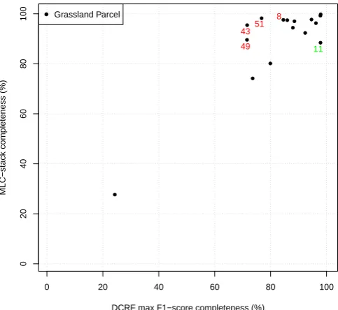
We further analyzed the grassland class where our approach has the lowest correctness compared to MLC-stack. Fig. 7 depicts completeness computed from each grassland validation parcel. Parcel numbers 8, 43, 49, and 51 have higher accuracy in MLC-stack compared to DCRF max F1-score. However, observations from ground referencing photos in Fig. 8 demonstrate that errors encountered by DCRF max F1-score in those parcels are true pos-itives. Hence, inhomogeneous grassland maps from DCRF max F1-score technique reflect true changes on ground not anticipated in ground reference data, see Fig. 8. Remaining parcels have comparable completeness accuracy in both methods.
A map of selected crops as classified by both MLC and DCRF max F1-score is shown in Fig. 9. It can be seen from the maps that DCRF max F1-score technique produces homogenous parcels compared to MLC-stack. This emphasizes the contribution of temporal phenological information inherent in images and spa-tial context in crop classification. The final map generated from DCRF max F1-score classification is illustrated in Fig. 10.
5. DISCUSSION
This study developed a DCRF crop classification technique from a sequence of TerraSAR-X images. In any classification, feature selection reduces computation demands. We selected four im-portant features according to RF for crop classification. Features from VV-polarization were found important in crop discrimina-tion compared to HH-polarizadiscrimina-tion as also established in Bargiel
● ● ●
●
●
●
●
● ●
● ●
●
● ●
●
●
0 20 40 60 80 100
0
20
40
60
80
100
DCRF max F1−score completeness (%)
MLC−stack completeness (%)
● Grassland Parcel 8
49 11
4351
Figure 7. Scatterplot of DCRF max F1-score against MLC-stack completeness computed each grassland validation parcel.
Figure 8. Grassland parcels as classified by MLC-stack and DCRF max F1-score and corresponding ground referencing photos. Top to bottom row corresponds to parcel numbers 49, 8,
and 11 respectively as shown in Fig. 7. Grey and white areas correspond to grasslands and misclassifications respectively.
and Herrmann (2011). We exploited their synergy for crop clas-sification. Our DCRF framework introduces spatial and temporal interactions. To enhance better data dependent spatial interac-tions we developed a new interaction term expanded from con-trast sensitive model. Experimental results established that our new model is robust and suitable for crop classification. We set
Figure 9. Maps of selected crops: top to bottom row represent oats, sugar beet, and maize parcels respectively. Correctly
classified regions are illustrated in grey colour.
±
Datum: WGS84 Projecttion: UTM Zone: 32N
1 0.5 0 1
km
Legend
Validation set Training set Barley Canola Grassland Maize
Oat Potato Rye Sugar beet Wheat Non Agricultural Area
Figure 10. Crop map of Fuhrberg, Germany, from DCRF Max-F1 approach . Crop legend adopted from Ebinger (2012).
discontinuity adaptive model that moderates smoothing consider-ing data evidence as suggested by Li (1995). Our model is
differ-ent from contrast sensitive model which only favours smoothing similar adjacent labels.
The novel interaction potential model is adopted in CRF to de-sign a DCRF sequence template classifier that considers inherent phenology in images. We established that including spatial and temporal phenological information improved classification accu-racy in all epochs. Moreover, our technique still outperformed MLC and CRF classification methods utilizing merged multitem-poral images as bands for classification (Table 2). To avoid a limited judgement using overall accuracy, we further compared our approach, DCRF max F1-score, with MLC using stacked im-ages. Analysis of correctness and completeness exposed a de-tailed distribution of how each crop is recognized. DCRF max F1-score poorly classified grassland parcels compared to MLC-stack. However, errors encountered by the method correspond to true ground changes that were not detected by MLC-stack for two reasons. First, MLC-stack classification places all features in one feature space which leads to a large variance that dominates small variations in a class. Two, DCRF max F1-score considers data and label dependent spatial interactions. This is supported by the fact that in a homogenous parcel, e.g. parcel number 11 in Fig. 8, DCRF max F1-score completely recognizes the parcel with higher accuracy than MLC-stack method, see Fig. 7. In ad-dition, artificial changes or natural changes , e.g. due to different variety of grassland and changes in farm management as depicted by parcel number 49 and 8 in Fig. 8 respectively, are detected in DCRF max F1-score. In contrast, MLC-stack is a pixel based ap-proach that ignores context. Thus, classification results from it are accompanied by ”salt and pepper” effect (Fig. 9). All other grassland parcels were classified comparably well in MLC-stack and DCRF max F1-score because they are managed in a common and unique way, and driven by economic preconditions.
The advantage of our ensemble classifier is that it can be used with any number of available images at any time of a season to get an estimate of crop coverage. Moreover, compared to other classifier combination strategies, the weighting we introduced to the ensemble improved classification. Therefore, it guarantees an optimal map in terms of accuracy. This is essentially beneficial to governments and related stakeholders in food security policy formulations and seeking alternative preventive measures. In ad-dition, agricultural stock market and traders can anticipate good years while insurers can accurately compute premiums and deter-mine compensations where necessary.
6. CONCLUSION AND OUTLOOK
Our aim was to show that spatial-temporal information from a se-quence of images improves crop classification. This was achieved by designing a DCRF classifier that realized spatial context and temporal phenological information exchange between nodes in a temporal neighbourhood. Spatial interaction significantly en-hanced spatial dependency minimizing ”salt and pepper” effect witnessed in MLC. The introduced data interaction term enforces a discontinuity adaptive model that moderates smoothing given data evidence.
On the other hand, stakeholder are not interested in several maps generated at each epoch in the same area. For them, statistics from one optimal map may be more relevant. Therefore, we de-signed a new ensemble approach based on F1-Score selection cri-teria and correctness weighting. The weighting schedule proved useful during integration of different classifier results.
is that a crop appears different at different times in satellite im-ages. However, in some instances like preparation and post har-vesting the backscatter is not entirely from the crops. Our future study will introduce phenological information from other exter-nal sources.
ACKNOWLEDGEMENTS
The project is funded by the German Federal Ministry of Educa-tion and Research (Project 50EE1326) and images provided by DLR.
REFERENCES
Bargiel, D. and Herrmann, S., 2011. Multi-Temporal Land-Cover Classification of Agricultural Areas in Two European Regions with High Resolution Spotlight TerraSAR-X Data. Remote Sensing3(5), pp. 859–877.
Blaschke, T. and Strobl, J., 2001. What’s wrong with pix-els? Some recent developments interfacing remote sensing and GIS.GeoBIT/GIS6(1), pp. 12–17.
Breiman, L., 2001. Random forests. Machine Learning45(1), pp. 5–32.
Buja, K. and Menza, C., 2013. Sampling Design Tool for ArcGIS - Instruction Manual. NOAA, Silver Spring, MD.
Deutscher Wetterdienst, 2012. ”Mittelwerte der Temperatur und des Niederschlags bezogen auf den aktuellen Standort”.http: //www.dwd.de. (2 Oct. 2015).
Ebinger, L., 2012. ”133 map categories! How the US Department of Agriculture solved a complex cartographic design problem”.
http://www.sco.wisc. edu/news/133-map-categories- how-the-us-department-of-agriculture-solved-a-complex-cartographic-design-problem.html. (2 Oct. 2015).
Forkuor, G., Conrad, C., Thiel, M., Ullmann, T. and Zoungrana, E., 2014. Integration of Optical and Synthetic Aperture Radar Imagery for Improving Crop Mapping in Northwestern Benin, West Africa.Remote Sensing6(7), pp. 6472–6499.
Fritz, T. and Eineder, M., 2009. TerraSAR-X Ground Segment Basic Product Specification Document. Technical report, Ger-man Aerospace Center.
Hastie, T., Tibshirani, R. and Friedman, J., 2011.The Elements of Statistical Learning: Data Mining, Inference, and Prediction. Springer Series in Statistics, 2nd edn, Springer.
Hoberg, T. and M¨uller, S., 2011. Multitemporal Crop Type Classification Using Conditional Random Fields and Rapid-Eye Data. In:ISPRS Workshop, Hannover, Germany.
Kenduiywo, B., Bargiel, D. and Soergel, U., 2015. Spatial-Temporal Conditional Random Fields Crop Classification from Terrasar-X Images.ISPRS Annals1, pp. 79–86.
Kenduiywo, B., Tolpekin, V. and Stein, A., 2014. Detection of built-up area in optical and synthetic aperture radar images using conditional random fields. Journal of Applied Remote Sensing8(1), pp. 083672–1 – 083672–18.
Kittler, J., Hatef, M., Duin, R. and Matas, J., 1998. On combining classifiers.IEEE T. Pattern Anal.20(3), pp. 226–239.
Kumar, S., 2006. Discriminative random fields. Int. J. Comput. Vis.68(2), pp. 179–201.
Lafferty, J. D., McCallum, A. and Pereira, F., 2001. Conditional random fields: probabilistic models for segmenting and label-ing sequence data. In: 18th ICML, Morgan Kaufmann, San Francisco, CA, USA, pp. 282–289.
Leite, P., Feitosa, R., Formaggio, A., da Costa, G., Pakzad, K. and Sanches, I., 2011. Hidden Markov Models for crop recognition in remote sensing image sequences. Pattern Recognit. Lett.
32(1), pp. 19–26.
Li, S., 1995. On discontinuity-adaptive smoothness priors in computer vision.IEEE T. Pattern Anal.17(6), pp. 576–586.
Murphy, K., Weiss, Y. and Jordan, M., 1999. Loopy Belief Propagation for Approximate Inference: An Empirical Study. In: 15th Conference on Uncertainty in Artificial Intelligence, Morgan Kaufmann Publishers Inc., San Francisco, CA, USA, pp. 467–475.
OpenCV, 2014. Random Trees. http://docs.opencv.org/ modules/ml/doc/ml.html. (20 Nov. 2014).
Ozdarici-Ok, A., Ok, A. and Schindler, K., 2015. Mapping of Agricultural Crops from Single High-Resolution Multispectral Images—Data-Driven Smoothing vs. Parcel-Based Smooth-ing.Remote Sensing7(5), pp. 5611–5638.
Roscher, R., Waske, B. and F¨orstner, W., 2010. Kernel Discrim-inative Random Fields for land cover classification. In:IAPR Workshop on Pattern Recognition in Remote Sensing, pp. 1–5.
Shotton, J., Winn, J., Rother, C. and Criminisi, A., 2009. Texton-Boost for Image Understanding: Multi-Class Object Recogni-tion and SegmentaRecogni-tion by Jointly Modeling Texture, Layout, and Context.Int. J. Comput. Vis.81(1), pp. 2–23.
Siachalou, S., Mallinis, G. and Tsakiri-Strati, M., 2015. A Hid-den Markov Models Approach for Crop Classification: Link-ing Crop Phenology to Time Series of Multi-Sensor Remote Sensing Data.Remote Sensing7(4), pp. 3633–3650.
Sokolova, M., Japkowicz, N. and Szpakowicz, S., 2006. Beyond Accuracy, F-Score and ROC: A Family of Discriminant Mea-sures for Performance Evaluation. In: Advances in Artificial Intelligence, Lecture Notes in Computer Science, Vol. 4304, Springer-Verlag Berlin Heidelberg, pp. 1015–1021.
Sonobe, R., Tani, H., Wang, X., Kobayashi, N. and Shimamura, H., 2014. Discrimination of crop types with TerraSAR-X-derived information.Physics and Chemistry of the Earth, Parts A/B/C.
Sutton, C., McCallum, A. and Rohanimanesh, K., 2007. Dy-namic conditional random fields: Factorized probabilistic models for labeling and segmenting sequence data. Journal of Machine Learning Research8, pp. 693–723.
Swain, P. H., 1978. Bayesian Classification in a Time-Varying Environment.IEEE T. Syst. Man. Cyb.8(12), pp. 879–883.
Tilman, D., Balzer, C., Hill, J. and Befort, B., 2011. Global food demand and the sustainable intensification of agriculture.
Proceedings of the National Academy of Sciences 108(50), pp. 20260–20264.
World-Bank, 2011. ”Food Price Watch”.
http://www.worldbank.org/foodcrisis/