Agricultural and Forest Meteorology 105 (2000) 161–183
Spatial and temporal properties of water vapor and
latent energy flux over a riparian canopy
D.I. Cooper
a,∗, W.E. Eichinger
b, J. Kao
a, L. Hipps
c, J. Reisner
a,
S. Smith
a, S.M. Schaeffer
d, D.G. Williams
eaLos Alamos National Laboratory, MS J577, Los Alamos, NM 87545, USA bUniversity of Iowa, Iowa City, IA, USA
cUtah State University, Logan, UT, USA dUniversity of Arkansas, Fayetteville, AR, USA
eUniversity of Arizona, Tucson, AZ, USA
Abstract
A scanning, volume-imaging Raman lidar was used in August 1997 to map the water vapor and latent energy flux fields in southern Arizona in support of the (Semi-Arid Land Surface Atmosphere) SALSA program. The SALSA experiment was designed to estimate evapotranspiration over a cottonwood riparian corridor and the adjacent mesquite-grass community. The lidar derived water vapor images showed microscale convective structures with a resolution of 1.5 m, and mapped fluxes with 75 m spatial resolution.
Comparisons of water vapor means over cottonwoods and adjacent grasses show similar values over both surfaces, but the spatial variability over the cottonwoods was substantially higher than over the grasses. Lidar images support the idea that the enhanced variability over the cottonwoods is reflected in the presence of spatially coherent microscale structures. Interestingly, these microscale structures appear to weaken during midday, suggesting possible evidence for stomatal closure. Spatially resolved latent energy fluxes were estimated from the lidar using Monin–Obukhov gradient technique. The technique was validated from sap-flow flux estimates of transpiration, and statistical analysis indicates very good agreement (within
±15%) with coincident lidar flux estimates. Lidar derived latent energy maps showed that the riparian zone tended to have the highest fluxes over the site. In addition, the spatial variability of 30 min average fluxes were almost as large as the mean values. Geostatistical techniques where used to compute the spatial lag lengths, they were found to be between 100 and 200 m. Determination of such spatially continuous evapotranspiration from such a complex site presents watershed managers with an additional tool to quantify the water budgets of riparian plant communities with spatial resolution and flux accuracy that is compatible with existing hydrologic management tools. © 2000 Elsevier Science B.V. All rights reserved.
Keywords:Raman lidar; Geostatistical techniques; Monin–Obukhov gradient technique
1. Introduction
Measuring fluxes from the surface to the atmosphere over complex terrain and plant canopies challenges
∗Corresponding author.
the technological resources of both the meteorologi-cal and hydrologimeteorologi-cal sciences (Kaimal and Finnigan, 1994). The flux of water vapor associated with evapo-transpiration (ET) is one of the critical components of both water and energy balance models of hydrologi-cal systems. Strong variations in both space and time
over a wide range of scales compound the difficulties of understanding the role ET plays in both physical and biological systems.
To examine these variations, the Los Alamos National Laboratory’s volume-imaging water-vapor Raman lidar system was used to estimate the latent energy (LE) flux as a two-dimensional surface over the complex terrain of a riparian corridor. The LE flux was derived from lidar-measured water vapor and simultaneous point-sensor wind-field measurements integrated into a Monin–Obukhov (M–O) similarity scheme. Validation of the lidar derived LE fluxes uti-lized transpiration estimates obtained from sap-flow probes. While the use of M–O in complex terrain and heterogeneous surfaces is problematic, it is our initial attempt at mapping riparian zone ET with spatially continuous data.
This paper outlines the results of the data process-ing and analysis technique used to estimate the spa-tially resolved LE flux and its spatial variability over cottonwoods in a riparian corridor located in south-ern Arizona. These results represent a contribution of the Semi-Arid Land Surface Atmosphere (SALSA) experiment.
2. SALSA experimental description
2.1. Site and lidar overview
The Lewis Springs study site at the National Ripar-ian Conservation Area is in the semi-arid southeastern part of Arizona, near Sierra Vista and close to the bor-der of Mexico, at an elevation of 1250 m. The site is described in detail in Goodrich et al. (1998). The study site is bisected by the San Pedro river, which was flow-ing at approximately 0.05 m3s−1 during the
experi-mental period, 8 days in early August, 1997. The flow of the San Pedro was due to the summer monsoon rains of mid-July. During the study in early August, clouds were always present giving rise to variable incoming solar radiation (Williams et al., 1998). The vegetation at the study site consists of a grass-mesquite-sacaton association at higher elevations adjacent to the ripar-ian corridor and, within the corridor, two predominate species, Frémont cottonwoods (overstory) and Good-ding willows (understory). The riparian corridor veg-etation straddled both sides of the river to a width of
±50 to±150 m, depending upon the width of the first bench of the flood plain. Within the flood plain where the cottonwoods stand, the lateral elevation change was relatively small with little variation in topography, except within the narrow 4 m channel of the San Pedro. During August the cottonwood canopy was closed, oc-cluding the San Pedro river from above and fully shad-ing the ground almost everywhere on the flood plain. In order to compute LE fluxes from M–O similarity theory, it is necessary to consider the topography and landscape of the area of interest for two reasons: (1) the individual profiles were acquired at different ele-vations over complex terrain such that a given height relative to the ground could be different between individual scans; (2) profiles over trees must be ad-justed for the difference between the ground and the top of the canopy. The elevation and topographic data is used to derive the canopy height (h) that is subse-quently used to estimate the displacement height (d0)
and roughness lengths (z0). Lidar range-height scans
included negative angles that produced laser ground hits, whose return signals are 1–2 orders of mag-nitude higher than the atmospheric signal, allowing easy separation of the surface from the atmosphere. Since lidar scan position is both accurate and precise, the topographic surface composed of both ground and vegetation at the Lewis Springs site was mapped by the lidar with 1.5±0.75 m horizontal intervals and
0.1 m vertical accuracy. An elevation correction fac-tor was derived from the topographic “map” for each scan angle for later use in flux estimation. Details of the lidar processing and geometric corrections are in Eichinger et al. (2000).
The LANL Raman lidar, which creates volume images from two-dimensional scans of ranged lidar returns, was fielded with an array of various point sensors along the San Pedro river. The lidar data from the second site will be evaluated in future work. A complete description of the lidar, its operation, and its capabilities are in Eichinger et al. (1999). For ref-erence, the lidar has a range of about 700 m, a hori-zontal spatial resolution of 1.5 m, azimuthal scanning of 360◦, and a vertical step resolution as small as 0.05◦. The absolute accuracy of the lidar was shown to be±0.34 g kg−1at 95% confidence (Cooper et al.,
D.I. Cooper et al. / Agricultural and Forest Meteorology 105 (2000) 161–183 163
to quantify the grass–shrub vegetation ET properties. The data analysis from the second site will be pre-sented in a later study. A vertically pointing sodar was positioned at the edge of the cottonwood stand to pro-vide wind-field observations starting at the top of the 30 m canopy for later flux computations. Three-axis sonic anemometers and Krypton hygrometers were also placed at various sites to provide temporal obser-vations of surface wind patterns and latent heat fluxes.
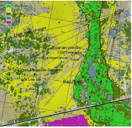
Fig. 1. Site map of the Lewis Springs study area compiled from a remotely sensed and classified image, showing the riparian zone in green, the grass-mesquite-sacaton association, location of the lidar, lidar lines-of-site, selected site instruments, and a major highway.
2.2. Wind-field data
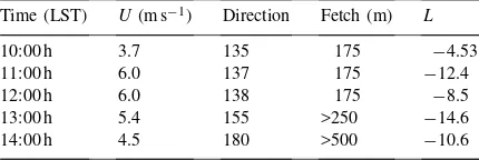
Flux estimates presented here were derived by combining the lidar data with wind-field observations from sensors distributed over the Lewis Springs study site. Wind-field data sets were obtained from cup anemometers and wind vanes over the grass region at 10 m height; from three-axis sonic anemometers at 2 m, and adjacent to the cottonwood canopy from a sodar system, which acquired horizontal (u, v), and verticalwwinds from heights of 25–600 m from the surface in 5 m increments. The wind direction during August 8 was somewhat parallel to the riparian corri-dor, between 120◦and 140◦for most of the morning and early afternoon, with the exception of midday when the wind changed abruptly (Fig. 2, Panel B). Wind speed continually increased during the morn-ing until it peaked at 6 m s−1 at 12:00 h LST and
thereafter began to drop again (Fig. 2, Panel C). Lidar estimates of LE flux using the M–O tech-nique require turbulence information in the form of friction velocity (u∗). Typical methods to obtain u∗ include either a mean wind profile or a three-axis sonic anemometer to measure the eddy covariance of the horizontal and vertical wind components. During SALSA, a sodar was used to derive u∗ directly ad-jacent to the cottonwoods using the spatial time-lag technique as described in the user manual (Remtech, 1994). It is assumed here that theu∗measurements at a single point are representative of the entire cotton-wood canopy since the sodar measurements used were made from 30 to 600 m above the surface. A com-parison of u∗ values over the cottonwoods by sodar and over the grass site from a three-dimensional sonic anemometer is shown in Fig. 2, Panel A. Theu∗ val-ues over the cottonwoods are up to two times those of the grass site, although there appears to be a general correlation (r2=0.79) in the temporal pattern during the day with major excursions occurring in the mid-afternoon. The assumption ofu∗as representative of a region is an area of future work.
3. Spatial properties of water vapor and water vapor flux
Preliminary analysis of the lidar data is presented here in two parts: (1) vertical lidar scans of water
vapor as a scalar, and (2) an analysis of lidar-derived spatial fluxes. The water vapor scalar analysis will fo-cus upon the relationship between observations over the riparian corridor versus the measurements over the adjacent grass–shrub communities. The analysis of the spatial properties of the LE flux will focus upon map-ping it, comparing the lidar-derived flux with coinci-dent sap-flow measurements, and analyzing its spatial variability.
3.1. Water vapor scalar properties of canopies
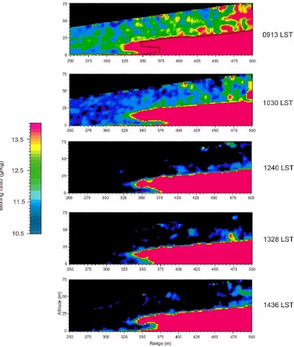
A cursory inspection of some of the lidar data re-veals interesting properties of the cottonwood canopy-surface layer interface when compared to the atmo-sphere above the relatively flat grass-mesquite-sacaton region adjacent to the riparian corridor. An example of a time-series of range-height lidar scans (here called vertical scans) acquired between 09:13 and 14:36 h LST on August 11, 1997 illustrates the spatial pat-terns and distribution of water vapor mixing ratio (q) in 1.5 m range-resolved pixels. The variations in color show red tones as highqvalues and blue tones as low qvalues (Fig. 3) (see Table 1 and Fig. 2 for wind di-rection). The vertical lidar images are composed of 42 individual scan lines where each scan required 0.75 s. Thus, it took about 32 s to complete and save each image. The time required to create an image might allow for substantial time–space distortion of the ob-served features. Work on a lidar simulation using a turbulence resolving model with 1.5 m resolution (see Kao et al., 2000; Fig. 4) indicates that the model can simulate the eddies from the cottonwood canopy, as well as simulate a 40 s scan by the lidar from the sur-face up into the atmosphere. The simulation indicates that the microscale convective structures (MCSs) ob-served by the lidar, even with time–space distortion,
Table 1
Fig. 3. Vertical lidar scans acquired between 09:13 and 14:36 h LST on August 11, 1997 showing the cottonwood canopy at 345 m range extending up to 30 m height above the surface. Azimuth of scans is at 195◦. Dotted line in the first panel (09:13 h LST) shows the
still show reasonable representations of these intermit-tent events, thus helping to validate the utility of the lidar derived data and images. Further, the model re-sults suggest that these structures should be coherent in space and time well past the lidar scanning period. The lidar return signal from the cottonwood trees was substantially larger than the atmospheric signal and saturates the detectors, therefore theqvalues from the leaves, stems, and trunks can be separated from the at-mospheric signal by using a simple threshold. By set-ting allqvalues above 16.8 g kg−1as “canopy” and all
values below 16.8 g kg−1as atmospheric signal, in the
images shown in Fig. 3, the canopy is solid red, and in the upper panel a dotted line has been added to de-note where the boundary between the canopy and the atmosphere is located. The dynamic range of the color table in Fig. 3 was optimized by fixing the range of the images between 10.5 and 14.0 g kg−1for the five
images to illustrate the effects of time on lower bound-ary moisture field. The black regions on the images are those areas where the water vapor mixing ratio is below the lowest color on the legend, 10.5 g kg−1.
When the return signal is less than 14.0 g kg−1,
pat-terns emerge from the data as can be seen in the un-stable regions above the surface and canopy (see Ta-ble 1 forLvalues). MCSs above the canopy are seen as “bubbles” of highqair presumably interacting with the relatively dryer air from above, such as the struc-ture at 430 m range and starting 30 m height acquired at 09:13 h LST. Inset C of Fig. 4 shows a horizon-tal transect (one line of sight) extracted from 37 m height from the 09:13 h LST vertical scan of Fig. 3, showing a ramp-like feature in the plume centered at 430 m. At 09:13 h LST the wind was nearly perpendic-ular to the lidar line-of-sight (Fig. 2B). Similar MCSs were observed by lidar over a green ash orchard that were closely related to intermittent features including “ramps” (Cooper et al., 1994). The highqfeatures over the mesquite-sacaton are 2–3 g kg−1 drier than those
over the cottonwood canopy. Interestingly, the appear-ance of these features were primarily in the morning hours and decrease in frequency until they disappear during midday; after about 13:30 h LST they begin to reappear again. While these MCSs are compelling, they must be interpreted with caution, as the lidar re-quires some time to acquire these images. Individual features such as those observed in Fig. 3 are com-posed of 15–25 lines-of-sight, take 10’s of seconds to
acquire, making these features spatially distorted and do not represent instantaneous images of convective structures. Further, the repeat rate for the same azimuth at this site was such that an evaluation of coherency directly from the lidar data is precluded. It is not clear at this time if these MCSs are due to dynamics above the canopy or canopy–atmosphere interactions such as sweep-ejection phenomena.
A more traditional method for displaying and analyzing the lidar data would be from vertical pro-files of water vapor extracted from the scans. One-dimensional profiles with 32 s averaging time were made by sorting the range pixels by their associ-ated height bins from an individual scan shown in the cross-sections shown in Fig. 3. Thus, all range pixels from a given region that fell into a speci-fied height range (e.g., from 0 to 0.5 m in eleva-tion) can be displayed as mixing ratio versus height. Two 25 m-wide sections were extracted from the 09:13 h LST scan in Fig. 3 at positions over both the grass-mesquite-sacaton association (at ranges be-tween 300 and 325 m in Fig. 3) and the cottonwoods (between 425 and 450 m). The grass was in the near field of the scan, limiting the height of the profile to 35 m. The sixteen 1.5 m lidar values per height bin in these 25 m scan widths give the data points of the profiles in Fig. 4. Although the average mixing ratio is similar for the two regimes, there is substantially larger variability at a given height over the cotton-woods. Both regimes exhibit an undulating structure with height, which reflects some of the coherent struc-tures visible in the image in Fig. 3. Fig. 4 suggests that the size of these structures are similar over both regimes, approximately 20 m. The plumes observed in Fig. 3 create the moistening observed 10–15 m above the canopy in the profiles of Fig. 4, as these plumes decay in height, the profiles show these higher regions as “dry”. It is interesting to note that only the lower portions of the profiles from single scans fit the Businger–Dyer semi-log model, while ensemble averaged profiles (over 30 min) smooth out most of these individual features and fit the semi-log model more completely (Eichinger et al., 2000).
D.I. Cooper et al. / Agricultural and Forest Meteorology 105 (2000) 161–183 169
is some 2.5 times greater for the cottonwoods than for the grass. While the deviations are pronounced, the lower portions of these profiles can be fitted to M–O predictions for mean gradients ofq (Eichinger et al., 2000).
Time-series of mean (q) and standard deviation (σq) values derived from vertically averaged 25 m tall subsections extracted from the water vapor distri-butions over both the grass and cottonwood canopy (from Fig. 4) are shown in Fig. 5. The mean values of qover the trees tend to be higher than over the grasses by modest differences of 0.5–1 g kg−1, although there
are periods when they are the same, most notably during midday. Coincident vapor pressure deficit measurements of cottonwood leaves at approximately 12:30 h LST also suggest reduced amounts of water vapor moving into the air, supporting the notion of stomatal control of water during high potential heat stress periods such as midday (Williams et al., 1998). As can be seen in Fig. 3, coherent plumes and struc-tures over the trees have deviations 2–3 g kg−1higher
than the background of 10.5–12 g kg−1, whereas over
the grass, the structures are somewhat weaker in in-tensity. This is because the well-watered trees are gen-erally transpiring at a higher rate than the dry grass, with the exception of midday, giving rise to more pronounced coherent structures. The σq time-series in Fig. 5 show that the atmosphere over the trees is al-ways more variable than over the grasses. The higher intensity turbulence over the trees (Fig. 2A) would explain the variability of the water vapor profiles over the cottonwoods as compared to the grasses. The cottonwood water-vapor variability was highest in the early afternoon between 12:00 and 13:30 h LST; thus LE fluxes are also expected to peak at the same time.
3.2. Microscale advective transport from the cottonwoods
The cottonwood stand is about 25 m taller than the surrounding grass-mesquite-sacaton association, cre-ating a roughness element change on the landscape with a unique microclimate environment. The effect of this microclimate on horizontal flow and ET is not well understood because measurement techniques generally rely on vertical transport or gradients. Li-dar data, combined with a soLi-dar point sensor is used
here to improve the understanding of the spatial and temporal properties of the three-dimensional canopy– atmosphere system.
The changing wind direction around midday in-creased the horizontal transport of mass and energy out of the cottonwoods and into the surrounding envi-ronment. The effects of wind on canopy transport can be seen in passive tracers such as the water vapor ob-servations made with the lidar. For example, at 11:56 h LST on August 11, a vertical scan was acquired when the wind direction was from the southwest (185◦), al-most directly facing into the lidar field-of-view. The lidar derived image suggests horizontal flow of water vapor out of the cottonwood canopy (Fig. 6). On this lidar image, the structure from the edge of the canopy, at 15 m from the ground, shows large concentrations of water vapor billowing off the cottonwood crowns horizontally into the lower surface layer over the grass. To better visualize this phenomenon, two 25 m-wide vertical water vapor profiles where extracted from this scan at 300 m range (Fig. 7A, over grass, “clear” air) and 320 m range (Fig. 7B, over grass, adjacent to the canopy). These profiles show the effects of horizontal transport from the canopy (Fig. 7). The mean water vapor from profile A is about 9.5 g kg−1in contrast,
the mean from profile B is closer to 11 g kg−1due to
D.I. Cooper et al. / Agricultural and Forest Meteorology 105 (2000) 161–183 173
numbers of point sensors are used to characterize the plant community.
3.3. Water vapor flux method
The LE flux estimates from lidar-measured vertical profiles of water-vapor mixing ratio use an M–O gra-dient driven similarity model. The traditional method for initializing this model would be to acquire verti-cal gradients of temperature, humidity, and wind from point-sensor time-series data and assume Taylor’s hy-pothesis of frozen turbulence to average over some user-defined region such as an agricultural field or vegetation surface cover type. The method used here employs the scanning and range resolving capabilities of the lidar to measure the spatially resolved vertical gradient of water vapor, and integrate these gradients with turbulence data to estimate a flux.
Earlier studies on the estimation of LE flux from lidar used water-vapor profiles aggregated from an entire site (Eichinger et al., 1992). These estimates were compared with eddy covariance and Bowen ra-tio derived flux values and found to be in excellent agreement. Here, we further extend this approach by incorporating a correction for topography on the li-dar cross-sections and combine several cross-sections into discrete spatial elements which are basically the mapping units that are then adjusted for displacement and roughness heights. This extension assumes that the statistics acquired over space can be averaged over time. By breaking down the site into discrete spatial elements, complex terrain becomes more accessible to M–O approaches for estimating fluxes. The next ques-tion is how big should the sampling size be?
Our previous work on the spatial variability of uniform vegetated surfaces indicates that the average scalar spatial structure (lags) size near the surface for water vapor is on the order of 10–20 m (Cooper et al., 1992). Similar lags of 10–15 m were also found over open water (ocean) surfaces as well (Cooper et al., 1997). Analysis of horizontal water vapor scans over the riparian corridor from this experiment support the earlier work, with spatial lags under 25 m (inset B, Fig. 10). Using the water vapor scalar structure size estimated from the variogram analysis and the compromise of the smallest possible statistically sig-nificant sample as criteria, we used a 25 m×25 m region as our initial flux mapping element. In essence,
we are assuming that within a 625 m2 area, Taylor’s
hypothesis is valid; that the grid element is spatially homogeneous and temporally stationary. These as-sumptions concerning the spatial element size of LE flux are still open to debate, and geostatistical tech-niques on the data collected from the SALSA experi-ment will explore part of this problem in Section 3.6. Estimates of ET from the Lewis Springs study site was generated by integrating wind-field data from a sodar with water vapor gradients derived by lidar. Li-dar vertical scans were typically 500–600 m long and extended up to 75 m in height above the canopy which is approximately 2–2.5 times the height of the cot-tonwood trees, Simpson et al. (1998) considered this range ideal for gradient measurements over forested sites. The vertical profiles used for flux mapping ex-tended up to 15 m above the canopy. The scans were stepped every 5◦ in azimuth, to form a swath up to 120◦wide used to create 30 min averaged flux maps. The first 100 m of lidar data (in range) are excluded from the analysis due to the limited height of the available profiles and field-of-view issues of the lidar. Each 625 m2flux mapping element was composed of several hundred lidar water vapor observations, giv-ing good statistical confidence to the gradients mea-sured between the canopy and atmosphere. The ripar-ian zone was mapped for a given 30 min period with several (up to three) sequences of scans starting at the south and progressing north by 5◦ increments. These scan series required 20–30 min; therefore the flux data on the maps can have a average time lag of±15 min across the flux map. The effect of this time lag on LE flux uncertainty is not precisely known at this time, but apparently is not large as evaluated by data simu-lation studies over the SALSA site (Kao et al., 2000). The landscape was partitioned into 25 m×25 m grid units that were based upon the lidar polar coordinate scan pattern, and became the spatial basis for M–O derived LE flux maps shown in the next section. Ver-tical water-vapor data that fell within a given map unit were then aggregated from the 1.5 m×1.5 m by 0.1◦ vertical data values into spatially discrete profiles typ-ically between 5 and 15 m in height for flux computa-tion. These profiles were then corrected for terrain and canopy height using lidar-derived topographic data and adjusted ford0andz0. The re-mapped water-vapor
(Brutsaert, 1982). The water vapor profile is given by
where qz is the water vapor mixing ratio measured by the lidar at some height above the surface;qs the
water vapor mixing ratio measured by the lidar close to the surface; L the latent heat of vaporization; E the latent heat flux to be calculated; av the ratio of
Von Karman’s water vapor constant to Von Karman’s constant,k;u∗the friction velocity from the sodar;ρ the air density;zthe measurement height;d0 the
dis-placement height derived from canopy height;z0 the
roughness length also derived from canopy height; ψsv(ζ) is the stability correction (Paulson, 1970).
Specific equations for the unstable atmospheric condition are found in Brutsaert (1982), and details on LE,L, andψsv(ζ) computation are in Eichinger et al.
(2000). LE flux is derived from Eq. (1) by algebraic re-arrangement following Eq. (1) through 6 of Eichinger et al. (2000). The basic 25 m×25 m LE flux map elements were then placed into a two-dimensional surface visualization software package to graphically smooth, display, and map the values as color coded maps of LE, where blue represents low LE values and red represents high LE values. Before the maps were completed a 3×3 nearest neighbor smoothing
algo-rithm was applied to the LE data, effectively reducing the spatial resolution of the LE maps to 75 m×75 m.
3.4. Limitations on the present lidar flux technique
M–O flux methods are most appropriate for sur-faces of uniform cover, flat terrain, stationary scalars and adequate fetch. These atmospheric conditions are rarely — if ever — met in the natural environment, not even over the open ocean where the surface is uniform (Fairall et al., 1996). As a consequence of these limi-tations, researchers either try to find sites that closely represent ideal conditions or modify their technique to account for the deviations from theory with the knowledge that the resulting fluxes have constraints associated with their interpretation. The fluxes derived using lidar data over the complex terrain of the San Pedro riparian zone are problematic but represent the best approach the authors have for estimating spatially resolved ET.
The problems with the lidar flux technique involve variations in roughness, spatial and temporal sam-pling, the use of uniform wind fields, as well as devi-ations from assumed profile theory. The most notable problem is the edge effect between the grasses and the cottonwoods as there is an approximately 30 m step change in roughness elements between the two vegeta-tion types. The present M–O approach is not designed to handle abrupt changes in elevation thus, flux values at these boundaries are suspect. A critical assump-tion for the lidar technique is that the 75 m×75 m (5625 m2) area where the water vapor profiles are measured is adequately sampled in space and time. Analysis of temporal sampling from point sensors suggests that the 30 min averaging period per flux estimate should be adequate under moderate winds. Temporal-spatial analysis also points to the potential of using footprint analysis to determine sampling size, frequency, and averaging period for the lidar as the technique becomes more refined (Horst, 1999; Schmid and Lloyd, 1999). Footprint analysis from BOREAS suggests that the flux fetch requirements could be on the order of 100 m×100 m (Kaharabata et al., 1997) under unstable conditions, although at a height of 16 m, Baldocchi (1997) reports that the entire footprint is about 80 m, suggesting that a 75 m×75 m sample size appears to be marginally adequate. While these studies are over different surfaces than SALSA, they support the contention that vertical coupling in the surface layer helps to reduce footprint areas. However, footprint methods predict the scalar back-trajectories to a tower (point) while the lidar incorporates a three-dimensional (x, y, z) region to estimate LE flux. The use of the lidar-measured volumetric source (albeit distorted over time) is assumed here to further reduce the footprint requirements to the order of the mapping elements shown in this paper; although this assumption is under investigation as an area of addi-tional study. The question of the source area footprint for LE flux and its relationship to lidar-measured pro-file thickness is a area of study that is ongoing and future work will attempt to address this issue.
D.I. Cooper et al. / Agricultural and Forest Meteorology 105 (2000) 161–183 175
resolved u∗ methods available, nevertheless it is the only assumption that can presently be made. It is hoped that three-dimensional mapping wind senors will be devised to evaluate this question in the future. Some tests can be applied to the data to determine how well it fits other aspects of theory, such as the semi-log profile of scalars [qz−qs is directly proportional to
ln(z−d0/z0), see Eq. (1)]. In particular, Eichinger
et al. (2000) shows that the lidar derived mean pro-files from SALSA fit theoretical predictions up to 30 or 40 m above the canopy, suggesting that the lidar data is not entirely outside the constraints of M–O theory.
3.5. Flux maps over the riparian corridor
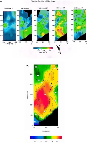
An M–O model (Eq. (1)) was used to compute LE fluxes from the data acquired on day 223 be-tween 10:00 and 14:00 h LST, and were subsequently mapped (Fig. 8). The stability and fetch conditions for the LE maps in Fig. 8 are shown in Table 1. The stability condition over the site on August 11 was highly unstable with z/L ranging from −8.5 to
−14.6, and the fetch was between 175 and 350 m. The patterns displayed on the five maps shown in Fig. 8a represent the ET over the riparian corridor and adjacent grass-mesquite-sacaton associations during midday. The highest flux values (red) in each map are loosely associated with the cottonwood stand, which runs roughly northwest to southeast at 100–200 m range, and the lower values (blue) adjacent to the riparian corridor represent LE values from the grass, and black represents no available data. The LE val-ues over the riparian corridor typically were between 50 and 350 W m−2, while the highest fluxes over the
grass typically exhibited only about half these values. The fluxes show relatively smooth iso-lines with few abrupt step changes in flux due to the continuous mix-ing by buoyant and mechanical processes in the lower parts of the surface layer (Kao et al., 2000). Unique patterns such as Panel D in Fig. 8a are apparently as-sociated with winds moving from the southeast to the northwest (Table 1). While the pattern of ET indicates that the riparian corridor typically displays higher ET than the (relatively dry) grass, the spatial distribution of LE values does not directly map over the vegeta-tion types, as there appears to be extensive mixing in the atmosphere, as discussed in Section 3.2. This
was not unexpected, because LE flux is a time–space averaged ensemble of various microscale intermittent atmospheric structures and larger scale processes, blending the boundaries of surface cover changes — which would suggest that horizontal mixing in the surface layer above the canopy plays an important role in the riparian ET process (Desjardins et al., 1992; Holwill and Stewart, 1992; Ogunjemiyo et al., 1997). Previous work on the issue of spatial variations in ET indicates that, not surprisingly, canopy heterogene-ity also contributes to flux variabilheterogene-ity (Tuzet et al., 1997). The range of late morning to mid-afternoon LE fluxes across the mapped region was between 15 and 350 W m−2 (or 0.02–0.46 mm h−1 of wa-ter), peaking during the 13:00–13:30 h LST period at over 330 W m−2. Average LE during the late
morning to mid-afternoon was about 230 W m−2 (or
0.30 mm h−1). In addition, the maximum variations in
LE flux across the mapped area occurred during the 13:00–13:30 h LST time period corresponding to high winds and incoming solar radiation. Total ET for the period between 10:00 and 14:00 h LST was mapped by summing the LE values from each of the 30 min maps shown in Fig. 8a and converting the LE units into depth units as shown in Fig. 8b. The riparian zone shows up in the image as high ET, up to 2.9 mm for this 5-h period, whereas the grass surrounding the cot-tonwoods showed somewhat smaller ET between 1.2 and 2.0 mm. To frame the size of the midday fluxes the total transpiration flux (by the sap-flow technique; Schaeffer and Williams, 1998) for the riparian corri-dor on day 223 was estimated at 5.2±0.4 mm; thus midday LE fluxes represent about half of the daily total ET.
3.6. Validation of flux technique
D.I. Cooper et al. / Agricultural and Forest Meteorology 105 (2000) 161–183 177
site map (Williams et al., 1998). The intercompar-ison data is presented in Fig. 9. Transpiration was estimated for nine cottonwood and six willow trees over 3–5 day periods using the heat pulse veloc-ity method (Cohen et al., 1981). The configuration of sap-flow probes provided estimates of sapwood area-based transpiration at 30 min intervals contin-uously over the periods covered by the intensive field campaign. Sapwood area-based transpiration measurements were combined with forest structural data (i.e., tree diameter, sapwood area-to-diameter relationships, and species composition) to estimate canopy area-based transpiration (in units of W m−2) for several multi-species tree clusters within the li-dar field-of-view. Tree clusters ranged from 444 to 1985 m2 in aerial cover and were situated both on
the forest margin and interior. The intercomparison is based upon transpiration estimates from the four tree clusters located in the interior of the riparian forest in order to avoid edge effects at the margins of the ripar-ian zone (Schaeffer and Williams, 1998). Edge effects were independently observed on thermal images of the site showing that the western edges were hotter than the rest of the canopy. These “hot spots” presum-ably have an effect on ET variability (Moran et al., 1998).
Uncertainties for the sap-flow estimates shown in Fig. 9 were derived from the re-examination of exist-ing comparison studies between the eddy correlation technique and coincident sap-flow flux observations (Hogg et al., 1997). Intercomparisons between the sap-flow and eddy covariance techniques show that sap-flow measurement variability is upward of±20%, and that differences between methods is±10% when there is no precipitation (Soegaard and Boegh, 1995). The lidar flux uncertainty estimates were derived from a comparison between drag coefficient methods (Fairall et al., 1996) and the lidar method (Eichinger et al., 1999). The uncertainty analysis presented by Eichinger et al. (2000) and the previously published uncertainty of 15% are consistent. The statistical com-parison, using a least-square regression between the sap-flow and lidar LE values yielded an r2 =0.89,
slope = 0.87, intercept = +19.3 W m−2, the RMS
error is±22 W m−2. On Fig. 9 many of the
intercom-parisons do not use site 251, the distance between site 251 and the lidar was close to the limit of the signal-to-noise for the system, consequently many of the
flux maps did not have values at this sap-flow gage. The RMS error is used here to represent an estimate of the sensitivity of the technique when compared to direct measures of transpiration, such as the sap-flow velocity method, assuming that this is an ideal tech-nique. The statistical analysis indicates that the lidar derived LE estimates are in good agreement with in situ observations, in spite of the numerous limitations of the present technique. However, until further exper-iments are evaluated and reported, these values must be interpreted with some caution. The sensitivity of
±22 W m−2appears to be adequate to separate fluxes
from two distinct vegetation types such as between the cottonwoods and the grass-mesquite-sacaton environ-ments. Lidar–sap-flow comparisons neither support nor refute the earlier findings that the sap-flow method overestimates LE in the morning and underestimates LE in the afternoon (Hogg et al., 1997). However, their does appear to be a small bias between the lidar and sap-flow estimates. Differences of 10–20% be-tween tree transpiration and evapotranspiration were also observed by Granier et al. (1990). Differences between eddy correlation and sap-flow derived fluxes are also consistent with the intercomparison data, fur-ther supporting the idea that it is possible to partition ET into transpiration and evaporative fluxes (Diawara et al., 1991). However, with the available instruments and techniques the inherent uncertainties are still too large to justify a statistically significant partitioning of LE fluxes.
3.7. Geostatistical analysis of water vapor scalar and flux
(1992) as
whereγij is the spatially dependent variance for spa-tial lagij,N(h) the number of paired vectors, andvare the data values at spatial location pointijin Cartesian coordinates. Once the variances are computed for all possible spatial lags, the variance is plotted as a func-tion of lag length, and characteristic variograms de-velop. The patterns that form the variogram are fitted with standard models of spatial distribution such as a spherical or Gaussian equation. The model chosen to fit the flux variograms was Gaussian which was also used in our earlier studies of spatial variability of scalar water vapor data (Cooper et al., 1992). The choice of models is supported by statistical analysis of the flux data indicating that the distribution was normal, and further, the ET process itself is spatially continuous supporting a Gaussian model (Isaaks and Srivastava, 1989). One of the aspects of Gaussian distributed var-iograms is that the variance is relatively insensitive to initial lag lengths. Thus, at small separations data tends to be highly correlated, which is what is ob-served in the LE maps. The Gaussian fitted model is as follows:
whereγhis the fitted variance,cthe scaling variance, hthe range at which 95% of the variance is reached in the variogram,Rthe range, andkthe offset (Deutsch and Journel, 1992). The fluxes are not estimated at a point, but represent a discrete area of 625 m2. There-fore it was assumed that the variogram would not have zero variance at the origin. With these analysis constraints of a Gaussian distribution and a non-zero origin, variograms were computed from the values used to create the LE maps for five periods from the late morning to the mid-afternoon. These variograms, as well as Gaussian fits to the variogram data, are shown in Fig. 10.
The variograms do not begin at the zero origin; instead they have a discrete variance at 0 m lag, which represents the inherent variability of the fun-damental measurement unit of 625 m2. The square
root of this variance is then a one standard deviation
estimate of the spatial variability of LE fluxes. This estimate ranged from ±35 W m−2 to approximately ±80 W m−2presumably dependent upon biophysical
and meteorological conditions, although the size of the variance appears to be correlated with incoming solar radiation (photosynthetic photon flux density versus time, Fig. 10, inset A) as on August 11 cloud attenuation of solar radiation corresponded with the alternating variances in Fig. 10. Furthermore, earlier studies of the variability of water vapor scalar during cloud-free periods suggested a strong dependence upon time, which in retrospect was probably also related to incoming solar radiation (Cooper et al., 1992). Similar variability results from catchment scale watersheds was estimated from spatially modeled ET values by Famiglietti and Wood (1995) as well as microscale measurements from area-averaged fluxes in Kansas (Smith et al., 1992). Variations greater than these ranges might not be due to spatial vari-ability and could be related to intermittent turbulent exchange processes such as sweep-ejection between the canopy and the lower atmosphere. The asymptote where the variability becomes constant with range occurred between 125 and 175 m, thus a region with an area consisting of these lags represents a region of uniform variability. Scaling analysis over a boreal forest indicates that almost 23 of the LE flux contri-bution from aircraft-tower measurements occurred at scales of approximately 200 m (Desjardins et al., 1997). The size of the range was not dependent upon the variability of the data, but does represent the structure size for a given time period. This would suggest that in order to characterize this riparian zone ET, instrument separations should be less than 175 m if the spatial uncertainty is to be minimized. The ad-equacy of 5625 m2areas appears to be reasonable for flux estimation without spatial undersampling in this environment.
4. Conclusions
D.I. Cooper et al. / Agricultural and Forest Meteorology 105 (2000) 161–183 181
atmosphere interactions including vegetation type, available water, and atmospheric dynamics. Sorting out the contributions from each of these factors will be an area for future research.
The lidar-based similarity technique for mapping fluxes were used to estimate LE to 75 m×75 m areas with a range in excess of 500 m. The validation of the lidar-derived LE flux was based upon intercom-parisons with sap-flow velocimetry measurements of transpiration. The correlation between the two tech-niques was 0.89. Interestingly the difference between ET and transpiration are about 10–15%. If the lidar and sap-flow methods are correct, then the evapora-tive component of the total ET for this riparian com-munity is relatively small when compared to other uncertainties such as spatial variability. LE flux values ranged over the site from 15 to 390 W m−2by 13:00 h
LST, with the riparian corridor accounting for the highest flux values. The total daily spatially averaged cottonwood transpiration measured by both the lidar and sap-flow methods, was on the order of 6 mm per day. Natural spatial distribution of ET during day 223 had the equivalent of up to 5 mm per day, suggesting that spatial variability is an important consideration in water budgets. The range of midday fluxes during peak ET periods across the Lewis Springs landscape was between 0 and 0.53 mm h−1 depending upon
location, while the range of fluxes solely within the riparian corridor was somewhat less, between 0.02 and 0.27 mm h−1.
Microscale horizontally advected transport of water vapor from the relatively tall and narrow cottonwood canopy may be important, and is not accounted for in the present similarity approach, and more work is needed to understand non-vertical transport of mass and energy. The lidar flux technique is sen-sitive enough to separate the ET from the riparian corridor and the grass-mesquite-sacaton areas. The spatial properties of the LE fluxes are somewhat de-pendent upon vegetation patterns, but it appears that atmospheric mixing is as important as surface cover type. Estimates of LE spatial variability for 30 min averages represent up to 10–20% of the mean fluxes. Furthermore, the spatial lags are between 125 and 175 m regardless of time. The lags are independent of the diurnal variability, but are dependent upon the inherent structure size of the ET process over the Lewis Springs site. This suggests that point sensors
such as eddy correlation instruments separated by more than the lag length will be sampling different canopy–atmosphere phenomenon.
The lidar is a powerful tool to be used in a suite of instruments for characterizing and mapping water vapor over non-homogeneous surfaces and complex terrain, and by extension we are taking the first steps in learning how to map the ET process as well. We will improve upon our understanding of the spatial pro-cesses involved in ET and the techniques to estimate fluxes, and with time the lidar methods will evolve into better and more acceptable forms. It is hoped that in the near future watershed managers will have a tool to quantify the water budgets of riparian veg-etation communities with spatial resolution and flux accuracy that is compatible with existing hydrologic management tools. The data presented here on the spatial properties of ET represent an improved vision of riparian consumptive use in semiarid watersheds over the traditional single point measurements of the past.
Acknowledgements
We would like to thank Vickie Cooper for her inspi-ration and time, J. Archuleta and L. Tellier of LANL, D. Goodrich, B. Goff, and S. Moran for there help in the logistics of SALSA and the rest of the ARS staff. Support from the NSF-STC SAHRA (Sustain-ability of Semiarid Hydrology and Riparian Areas) un-der Agreement No. EAR-9876800) is also gratefully acknowledged. This work was performed and funded in part under DOE grant W7405-ENG-36.
References
Baldocchi, D., 1997. Flux footprint within and over forest canopies. Bound. Layer Meteorol. 85, 273–292.
Brutsaert, W., 1982. Evaporation into the Atmosphere. Theory, History, and Applications. Reidel, Dordrecht, p. 299. Cleugh, H.A., Hughs, D.E., Judd, M.J., 1998. A field and
wind tunnel study of the velocity and scalar fields around a windbreak. In: Proceedings of the 23rd Conference on Agricul-tural and Forest Meteorology, Albuquerque, NM. American Meteorology Society, Boston, MA, pp. 131–134.
Cooper, D., Eichinger, W., Holtkamp, D., Karl, R., Quick, C., Dugas, W., Hipps, L., 1992. Spatial variability of water transfer within the boundary layer vapor turbulent. Bound. Layer Meteorol. 61, 389–405.
Cooper, D., Eichinger, W.E., Hof, D., Jones, D., Quick, R., Tiee, J., 1994. Observations of coherent structures from a scanning lidar. Agric. For. Meteorol. 67, 137–150.
Cooper, D.I., Eichinger, W.E., Barr, S., Cottingame, W., Hynes, M.V., Keller, C.F., Lebeda, C.F., Poling, D.A., 1996. High resolution properties of the equatorial pacific marine atmospheric boundary layer from lidar and radiosonde observa-tions. J. Atmos. Sci. 53, 2054–2075.
Cooper, D.I., Eichinger, W., Ecke, R., Kao, J., Reisner, J., Tellier, L., 1997. Initial investigations of micro-scale cellular convection in an equatorial marine atmospheric boundary layer revealed by lidar. Geophys. Res. Let. 24, 45–48.
Desjardins, R.L., Schuepp, P.H., MacPherson, J.L., Buckley, D.J., 1992. Spatial and temporal variations of the fluxes of carbon dioxide and sensible and latent heat over the FIFE site. J. Geophys. Res. 97, 18467–18475.
Desjardins, R.L., MacPherson, J.L., Mahrt, L., Schuepp, P.H., Pattey, E., Neumann, H., Baldocchi, D., Wofsy, S., Fitzjarrald, D., McCaughey, H., Joiner, D.W., 1997. Scaling up flux meas-urements for the boreal forest using aircraft-tower combinations. J. Geophys. Res. 102, 29125–29133.
Deutsch, D.V., Journel, A.G., 1992. Geostatistical Software Library and User’s Guide. Oxford University Press, New York, p. 340.
Diawara, A., Loustau, D., Berbigier, P., 1991. Comparison of two methods for estimating the evaporation of a Pinus pinaster
(Ait.) stand: sap flow and energy balance with sensible heat flux measurements by an eddy covariance method. Agric. For. Meteorol. 54, 49–66.
Eichinger, W., Cooper, D., Holtkamp, D., Karl, R., Moses, J., Quick, C., Tiee, J., 1992. Derivation of water vapor fluxes from lidar measurements. Bound. Layer Meteorol. 63, 39–64. Eichinger, W., Cooper, D., Kao, J., Chen, L.C., Hipps, L., 2000.
Estimating of spatially distributed latent energy flux over complex terrain from a raman lidar. Agric. For. Meteorol. 105, 145–159.
Eichinger, W., Cooper, D.I., Forman, P.R., Griegos, J., Osborn, M.A., Richter, D., Tellier, L.L., Thorton, R., 1999. The develop-ment of a scanning Raman water-vapor lidar for boundary layer and tropospheric observations. J. Ocean. Atmos. Tech. 16, 1753–1766.
Fairall, C.W., Bradley, E.F., Rogers, D.P., Edson, J.B., Young, G.S., 1996. Bulk parameterization of air-sea fluxes for tropical ocean-global atmosphere coupled-ocean atmosphere responce experiment. J. Geophys. Res. 101, 3747–3764.
Famiglietti, J.S., Wood, E.F., 1995. Effects of the spatial variability and scale on areally averaged evapotranspiration. Water Resour. Res. 31, 699–712.
Goodrich, D.C., Chehbouni, A., Goff, B., MacNish, B., et al., 1998. An overview of the 1997 activities of the semi-arid land surface atmosphere (SALSA) program. In: Special Symposium on Hydrology, Phoenix, AZ. American Meteorology Society, Boston, MA, pp. 1–7.
Granier, A., Bobay, V., Gash, J.H.C., Gelpe, J., Saugier, B., Shuttleworth, W.J., 1990. Vapor flux density and transpiration rate comparisons in a stand of Maritime pinePinus pinaster
(Ait.) in Les Landes forest. Agric. For. Meteorol. 51, 309–319. Hogg, E.H., Black, T.A., Hartog, G.D., Neumann, H.H., Zimmermann, R., Hurdle, P.A., Blanken, P.D., Nesic, Z., Yang, P.C., Staebler, R.M., McDonald, K.C., Oren, R., 1997. A comparison of sap flow and eddy fluxes of water vapor from a boreal deciduous forest. J. Geophys. Res. 102, 28929–28937. Holwill, C.J., Stewart, J.B., 1992. Spatial variability of evaporation
derived from aircraft and ground-based data. J. Geophys. Res. 97, 18673–18680.
Horst, T.W., 1999. The footprint for estimation of Atmosphere-Surface Exchange Fluxes by Profile Techniques. Bound. Layer Meteorol. 90, 171–188.
Isaaks, E.H., Srivastava, R.H., 1989. An Introduction to Applied Geostatistics. Oxford University Press, New York, 561 pp. Kaimal, J.C., Finnigan, J.J., 1994. Atmospheric Boundary Layer
Flows. Oxford University Press, New York, p. 289.
Kao, C.-Y.J., Hang, Y.-H., Cooper, D.I., Eichinger, W.E., Smith, W.S., Reisner, J.M., 2000. High-resolution modeling of lidar data: mechanisms governing surface water vapor variability during SALSA. Agric. For. Meteorol. 105, 185–194. Kaharabata, S.K., Schuepp, P.H., Ogunjemiyo, S., Shen, S.,
Leclerc, M.Y., Desjardins, R.L., MacPherson, J.I., 1997. Foot-print considerations in BOREAS. J. Geophys. Res. 102, 29113– 29124.
Moran, S., Williams, D., Goodrich, D., et al., 1998. Overview of remote sensing of semi-arid ecosystem function in the upper San Pedro River Basin, Arizona. In: Special Symposium on Hydrology, Phoenix, AZ. American Meteorology Society, Boston, MA, pp. 49–54.
Ogunjemiyo, S., Schuepp, P.H., MacPherson, J.I., Desjardins, R.L., 1997. Analysis of flux maps versus surface characteristics from Twin Otter grid flights in BOREAS 1994. J. Geophys. Res. 102, 29135–29145.
Paulson, C.A., 1970. The mathematical representation of wind speed and temperature profiles in the unstable atmospheric surface layer. J. Appl. Meteorol. 9, 857–861.
Remtech Inc., 1994. DT94/003 Remtech Doppler Sodar Operating Manual; Appendix A, Software General Description. Remtech Inc., PO Box 2423, Longmont, CO, USA, p. 27.
Schaeffer, S.M., Williams, D.G., 1998. Transpiration of desert riparian forest canopies estimated from sap flux. In: Special Symposium on Hydrology, Phoenix, AZ. American Meteo-rology Society, Boston, MA, pp. 180–183.
Schaeffer, S.M., Williams, D.G., Goodrich, D.C., 2000. Transpiration of cottonwood/willow forest estimated from sap flux, Agric. For. Meteorol. 105, 257–270.
Schmid, H.P., Lloyd, C.R., 1999. Spatial representativeness and the location bias of flux footprints over inhomogeneous areas. Agric. For. Meteorol. 93, 195–209.
Simpson, I.J., Thurtell, G.W., Neumann, H.H., Den Hartog, G., Edwards, G.C., 1998. The validity of similarity theory in the roughness sublayer above forests. Bound. Layer Meteorol. 87, 69–99.
D.I. Cooper et al. / Agricultural and Forest Meteorology 105 (2000) 161–183 183 index and eddy correlation technique. J. Hydrol. 166, 265–
282.
Smith, E.A., Hsu, A.Y., Crosson, W.L., Field, R.T., Fritschen, L.J., Gurney, R.J., Kanemasu, E.T., Kustas, W.P., Nie, D., Shuttleworth, W.J., Stewart, J.B., Verma, S.B., Weaver, H.L., Wesely, M.L., 1992. Area-averaged surface fluxes and their time–space variability over the FIFE experimental domain. J. Geophys. Res. 97, 18599–18622.
Tuzet, A., Castell, J.F., Perrier, A., Zurfluh, O., 1997. Flux heterogeneity and evapotranspiration partitioning in a sparse canopy: the fallow savanna. J. Hydrol. 188, 482–493. Williams, D.G., Brunel, J.P., Schaeffer, S.M., Snyder, K.A.,