A GRAPH BASED MODEL FOR THE DETECTION OF TIDAL CHANNELS USING
MARKED POINT PROCESSES
A. Schmidt a, F. Rottensteiner a, U. Soergel b, C. Heipke a
a
Institute of Photogrammetry and GeoInformation, Leibniz Universität Hannover, Germany - (alena.schmidt, rottensteiner, heipke)@ipi.uni-hannover.de
b
Institute of Geodesy, Chair of Remote Sensing and Image Analysis, Technische Universität Darmstadt, Germany - [email protected]
KEY WORDS: Marked point processes, RJMCMC, graph model, digital terrain models, coast
ABSTRACT:
In this paper we propose a new method for the automatic extraction of tidal channels in digital terrain models (DTM) using a sampling approach based on marked point processes. In our model, the tidal channel system is represented by an undirected, acyclic graph. The graph is iteratively generated and fitted to the data using stochastic optimization based on a Reversible Jump Markov Chain Monte Carlo (RJMCMC) sampler and simulated annealing. The nodes of the graph represent junction points of the channel system and the edges straight line segments with a certain width in between. In each sampling step, the current configuration of nodes and edges is modified. The changes are accepted or rejected depending on the probability density function for the configuration which evaluates the conformity of the current status with a pre-defined model for tidal channels. In this model we favour high DTM gradient magnitudes at the edge borders and penalize a graph configuration consisting of non-connected components, overlapping segments and edges with atypical intersection angles. We present the method of our graph based model and show results for lidar data, which serve of a proof of concept of our approach.
1. INTRODUCTION
In general, strategies for the automatic detection of objects from images can be divided into top-down and bottom-up approaches. For the latter, basic image processing methods such as segmentation are employed and the results are assigned to scene objects afterwards. In contrast, top-down approaches integrate knowledge about the objects and search for matches with the input data. Stochastic methods such as marked point processes (Daley and Vere-Jones, 2003), which achieve good results in various disciplines, belong to the top-down approaches. Marked point processes do not work locally, but rather enable to find a global optimum of the configuration of objects. Model knowledge can be integrated in different ways. To this end Lafarge et al. (2010) developed a flexible approach for the detection of different kinds of objects in images. For that purpose, the authors set up a library composed of simple geometric patterns such as rectangles, lines and circles, which are defined by their lengths, orientations or radii. The geometric patterns are randomly fitted to the images and their conformity with the input data is evaluated based on the mean and standard deviations of the gray values inside and outside the proposed objects as well as the overlapping area between them. The authors achieve good results for different fields of application such as the extraction of line networks, buildings or tree crowns. Tournaire et al. (2007) used marked point processes for the extraction of dashed lines representing road markings from very high resolution aerial images. Here, the objects are modelled by rectangles whose conformity with the input data is evaluated based on the gray values of the pixels inside the rectangles and in their local neighbourhood. Both are modelled to be homogenous while pixels inside the rectangles have to have bright pixels. The authors penalize configurations in which the distance between rectangles differs from the expected one
depending on the road type. Road networks are extracted in the approach of Lacoste et al. (2005). This is done by taking into account different types of relations between segments and evaluating their connectivity and orientation. The input data are considered by calculating the homogeneity of the gray values of the road and the gray level variation between the road and the background. A similar approach was developed by Sun et al. (2007) for the automatic extraction of vessels on angiograms. The vessels are modelled as line segments; their configuration is optimized by penalizing segments which are not connected at both ends. The conformity with the input data is determined based on a vesselnessenhancement measure which is calculated from the two eigenvalues of the Hessian of the image function. Perrin et al. (2005) used marked point processes for the detection of tree crowns from remotely sensed images with infrared information in order to derive tree parameters such as the diameter or the density. The trees are modelled by ellipses whose overlapping area is penalized depending on the way they overlap. A further term is introduced in order to favour regular alignments in the configuration. Furthermore, extreme closeness of objects is penalized by a constant parameter.
We aim to take advantage of the benefits of marked point processes (the global optimization and their flexibility due to the fact that the approach is a stochastic one) in order to detect tidal channels in a digital terrain model (DTM) derived from lidar data. Tidal channels are a special type of rivers furrowing the mudflat areas in coastal zones. Because they have large impact on the sedimentation and the ecology of the flat coastal waters, a detailed understanding of their characteristics is essential. Moreover, they significantly change position over time due to the influence of the tides and storm events. Extracting them automatically from remote sensing data is a challenging task.
In our previous work, we developed a two-step approach for that purpose (Schmidt et al., 2014). First, we fitted rectangles to the data using marked point processes. High DTM gradient magnitudes on the rectangle borders and non-overlapping objects were introduced to model the tidal channels. In a second step, we determined the principal axes of the rectangles and their intersection points. Based on this result a graph was constructed in which nodes represented junction points or end points, respectively, and edges straight line segments located in between. While overall the results were promising, they revealed that the topology of the tidal channel network was not always correctly described. Furthermore, the connectivity of all channels was not guaranteed. That is why we intended to integrate this characteristic directly in the sampling process.
In this paper, we adopt the method of Chai et al. (2013) and modelled tidal channels by a graph and optimize its configuration. In the graph nodes represent junction points and edges correspond to straight line segments with a certain width. We integrate the evaluation criteria of our previous work into angles between adjacent edges which differ from those typically found in tidal channel networks.
We first describe the mathematical foundation of the stochastic optimization using marked point processes (Section 2). Then, we present the proposed graph based model for our application (Section 3). In Section 4, we show some experiments and results on test data of the German Wadden Sea. Finally, conclusions and perspectives for future work are presented.
2. THEORETICAL BACKGROUND
2.1 Marked point process
Point processes belong to the group of stochastic processes, a collection of random variables. They are used for the description of phenomena in which the random variable can be observed only at particular points of time (for random variables with temporal reference) or at particular locations (for random probable configuration of objects in a scene given the data. An object is described by its location li. In a marked point process, a mark mi, a multidimensional random variable, is added to each point describing an object of a certain type. If we characterise
There are different types of point processes. The Poisson point process ranks among the basic ones, it assumes a complete randomness of the objects, and the number ofobjects n follows a discrete Poisson distribution with parameter also called intensity parameter, which corresponds to the expected value
for the number of objects. In the Poisson point process, the objects are independent and uniformly distributed in S, given n.
In practice, a complete randomness of the object distribution is often not applicable. Instead, more complex models are postulated. However, they are described with respect to a reference point process, which is usually defined as the Poisson point process. In our model, we define the probability density introduces prior knowledge about the object layout; our models for these two energy terms are described in Section 3. The optimal configuration of objects can be determined by minimizing the Gibbs energy U(.), i.e.
. Since the number of possible object configurations increases exponentially with the size of the object space, the global minimum can only be approximated. This is done by coupling a RJMCMC sampler and a simulated annealing relaxation.
2.2 Reversible Jump Markov Chain Monte Carlo
Markov Chain Monte Carlo (MCMC) methods belong to the group of sampling approaches. The special feature of the method is that the samples are not drawn independently. On the contrary, each sample Xt, , has a probability distribution that depends on the previous sample Xt-1. Thus, the sequence of samples forms a Markov chain which is simulated in the space of possible configurations. If the number of objects constituting the optimal configuration were known or constant, MCMC sampling (Metropolis et al., 1953, Hastings, 1970) can be used for its determination. Reversible jump Markov Chain Monte Carlo (RJMCMC) is an extension of MCMC that can deal with an unknown number of objects and a change of the parameter dimension between two sampling steps (Green, 1995). In each iteration t, the sampler proposes a change of the current configuration from a set of pre-defined types of changes according to a density function. Each of the types is also associated with a density function Qi called kernel. Each kernel Qi is reversible, i.e. each change can be reversed applying another type of kernel. The type of changes and the kernels in our model are described in Section 3. A kernel Qi is chosen randomly according to a proposition probability which may depend on the kernel type. The configuration Xt is changed according to the kernel Qi, which results in a new configuration Xt+1. Subsequently, the Green ratio R (Green, 1995) is calculated:
In (2), Ttis the temperature of simulated annealing in iteration t (cf. Section 2.3). The International Archives of the Photogrammetry, Remote Sensing and Spatial Information Sciences, Volume XL-3/W3, 2015
Following Metropolis et al. (1953) and Hastings (1970) the new configuration Xt+1 is accepted with the probability α and rejected with the probability 1-α. The four steps of (1) choosing a proposition kernel Qi, (2) building the new configuration Xt+1, (3) computing the acceptance rate α, and (4) accepting or rejecting the new configuration are repeated until a convergence criterion is achieved.
2.3 Simulated Annealing
In order to find the optimum of the energy, the RJMCMC sampler is coupled with simulated annealing. For that reason, the parameter Tt referred to as temperature (Kirkpatrick et al., 1983) is introduced in equation 2. The sequence of temperatures
Tt tends to zero as . Theoretically, convergence to the global optimum is guaranteed for all initial configurations X0 if
Tt is reduced (“cooled off”) using a logarithmic scheme. In
practice, a geometrical cooling scheme is generally introduced instead. It is faster and usually gives a good solution (Salamon et al., 2002; Tournaire et al., 2010).
3. METHODOLOGY
We fit objects to the data using a RJMCMC sampler and simulated annealing as described in Section 2. Our model is based on our previous work (Schmidt et al., 2014) where we adapted the approach of (Tournaire et al., 2010) to our application of tidal channel detection in a DTM, but differs in the object model we use. Instead of rectangles, we now take into account the network structure of our object of interest (see Section 3.1) and optimized the configuration of an undirected graph. Following Chai et al. (2013), nodes in the graph represent junction points with outgoing segments varying in number and representing the tidal channels in the DTM. A segment becomes an edge in the graph if it links two nodes (Section 3.1). In the sampling process, nodes are iteratively added to or removed from the graph in order to find the best object configuration. Moreover, we allow for a modification of the node parameters. The changes of the configuration are described in Section 3.2. In each iteration we evaluate the graph configuration based on a global energy function which is minimized during the sampling process. Here, we favour high gradients at the segment borders and penalize the overlapping area of segments, segments which are not connected to the tidal channel system on both ends and angles between edges which differ from those typically found in tidal channel networks (Section 3.3).
3.1 Object model
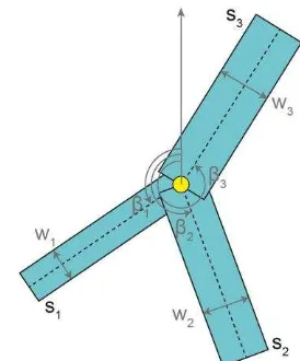
We characterize an object ui = (li, mi) by its location li=(x,y)and its parameters mi. In our approach, the objects are junction points similar to the approach of Chai et al. (2013). Each junction point possesses n outgoing segments sj (j = 1,..., n), each corresponding to a part of a tidal channel in the DTM (Fig. 1). The minimum number of segments is n = 1 (the junction point becomes an end-point in the network); it can rise to n = k
whereby k is the predefined maximum number of tidal channels converging on a junction point. We specify the segments by their directions (the counterclockwise angles βj relative to the positive y-axis) and their widths wj. In total, the junction point parameters are mi = (β1, ..., βn,w1, ..., wn).
Figure 1. The object in our configuration is a junction point with n outgoing segments (here: n = 3). Each segment sj is characterized by its width wj and its direction βj (the counterclockwise angle relative to the positive y-axis).
3.2 Changes of the configuration
We integrate four different types of changes in our approach. On the one hand, an object can be added to or removed from the current configuration, which is accomplished by the birth and death kernels, QB and QD, respectively. On the other hand, the parameters of an object of the current configuration can be modified. Here, we define the translation of a junction point which is equivalent to a change of its position (translation kernel QT) and the modification of one of its segment parameters (modification kernel QM). The type of changes and the associated kernels are described in more detail in the following section.
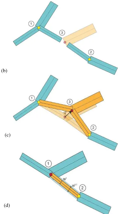
3.2.1 Birth event: For the birth event, the position and the number of segments of a new junction point are generated. It should be noted that all of the junction point parameters (position, number of segments, their directions and widths) may be generated based on learned probability density functions. The junction point is added to the graph as a node. Then, neighbouring junction points are determined in a local neighbourhood and the feasibility of adding an edge between them and the new node is checked. For that purpose, we integrate three criteria. First, we do not allow the segment corresponding to this edge to intersect with another edge in the graph. In this way, we take into account that tidal channels do not intersect without a junction point at the point of intersection. Second, we do not allow cycles in the graph, bearing in mind that water flows only in one direction (namely downhill). By building up an acyclic graph, we accept that we cannot detect two channels circling round an island. However, this particular case rarely occurs in our application. Third, we introduce a threshold for the angle between two edges in order to avoid too much overlap of segments in a node. If a neighbouring node does not violate any of these criteria, we add an edge connecting it with the new node (Fig. 2a). The neighbouring nodes are considered in the order of their distance to the node. Finally, we modify the neighbouring node involved and add the new segment or replace an existing segment based on an angle criterion.
3.2.2 Death event: A junction point is randomly chosen and the corresponding node as well as its outgoing edges are removed from the graph. The neighbouring nodes retain a seg-ment in the direction of the removed node, however (Fig. 2b).
3.2.3 Translation event: A displacement vector for a (randomly chosen) node in the graph is randomly generated within a local neighbourhood. For outgoing edges we check for an intersection of the corresponding segment with the existing segments in the configuration and the angle to the other segments (similar to the criteria for the birth kernel). If these criteria are not violated, the junction point is translated and its position and directions are modified. We also update affected neighbouring nodes (Fig. 2c).
3.2.4 Modification event: We randomly choose a junction point and one of its segments and change its width (within predefined thresholds for the minimum and maximum width of a segment). If this segment corresponds to an edge, the neighbouring node is modified by updating the width for the corresponding segment (Fig. 2d) 1.
3.2.5 Kernels: In equation (2), the Green ratio is calculated based on the kernel ratio which takes into account the probability for the change of the configuration from Xt+1 to Xt and vice versa. Following Chai et al. (2013), we model the kernel ratio for the birth and the death events by
In (4) and (5) pD and pB correspond to the probability for
choosing a birth or death event, respectively. λ is the intensity value of the Poisson point process which serves as reference process in our model (cf. Section 2.1) and n is the current number of nodes in the graph.
For the translation and the modification event, we set the kernel ratio to 1:
1
Additional modifications are part of further research.
Figure 2: Four types of changes are defined for the sampling process. Nodes and segments which are chosen for a change are depicted in red and orange. The configuration before the change is depicted slightly transparent. The medial axes of the segments are illustrated by a solid line if they belong to an edge in the graph. (a) Birth kernel: Node 3 is added to the graph. Neighbouring nodes are connected by edges if they fulfil some criteria. Segments of the neighbouring nodes whose angle ω to the new direction is below a predefined threshold are removed (transparent segment of node 1). (b) Death kernel: Node 3 is removed from the configuration. Nodes 1 und 2 retain a segment in the direction of the removed node. (c) Translation kernel: The position ofnode 1 is changed by the displacement vector . Edges to neighbouring nodes are retained if they do not lead to crossing edges. (d) Modification kernel: The parameters of one of the outgoing segments of node 1 are changed. Because the segment belongs to an edge, the parameters of node 2 are changed, too.
3.3 Energy model
Each configuration is evaluated based on the Gibbs energy which is minimized during the sampling process. In our model, the Gibbs energy consists of two terms: the data energy and the prior energy. We set a maximum value for the length of those segments which do not correspond to an edge and, thus, do not have a neighbouring node.
(a)
(b)
(c)
(d)
3.3.1 Data Energy: The data energy Ud(Xt) (equation 1) checks the consistency of the object configuration with the input data. Tidal channels are characterized by locally smaller heights and have high DTM gradient magnitudes on each bank and flat gradient magnitudes between these banks in the areas that may or may not be covered by water (depending on the tides). We adapt and slightly modify the data term of our previous model (Schmidt et al., 2014) where we fitted rectangle to the data. Here, we determine the gradients of the segments borders by
weights. The normal vector is defined to point from the interior of the segment to the outside. We take into account only the two borders of the segment corresponding to the channel banks. A this way, the accumulation of objects in regions with high data energy can be avoided. Second, we aim to end up in a configuration with only one graph and, thus, rate the connectivity of the nodes in the graph. Third, we favour those angles between edges which typically occur within tidal channel networks. In total, the prior energy is modelled by
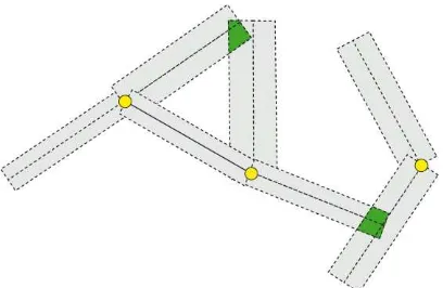
do not calculate the overlapping area of two segments belonging to the same node (Fig. 3).
In order to evaluate the connectivity of the graph, we penalize all segments which do not link two nodes by
where ns is the number of segments in the graph which are connected to only one segment and fs is a constant penalizing factor.
Finally, favouring certain angle configuration between two edges is achieved by edges is subtracted from the expected angle for typical tidal channel configuration which may be learned from the data or integrated as prior knowledge. fa is a constant penalizing factor.
Figure 3: The overlapping area for all pairs of segments is calculated if both segments do not belong to the same node. Here, the green areas correspond to our prior energy term.
4. EXPERIMENTS
4.1 Test data
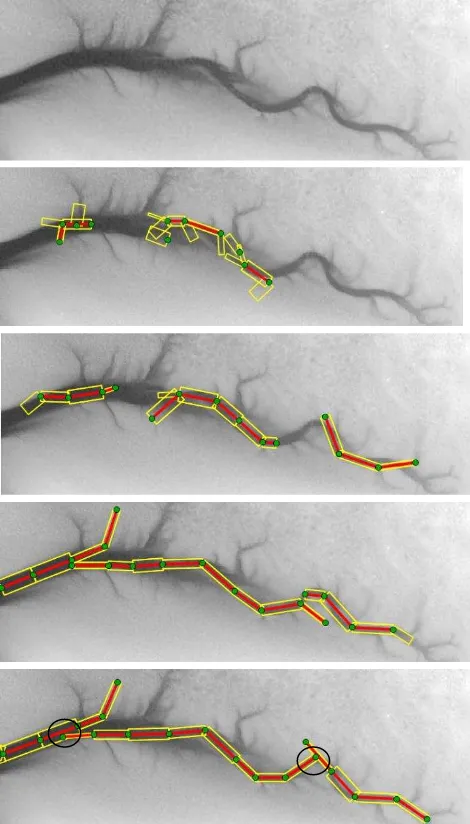
We evaluate our method on lidar data from the German Wadden Sea. The test site is located in the south of the East Frisian island Norderney and covers an area of 440 x 150 m2. The flight campaign took place in spring 2012 using a Riegl LMS-Q 560 sensor. The heights of the raw lidar point cloud (average point heights in our data and propose a new junction point in the birth event only at pixels whose height is below this threshold. The difference for both of the values and take the smaller one in our prior term. For junction points with three segments we set the minimum (Fig. 6). Then, the main tidal channel in the middle of the scene is nearly completely covered by segments. Most of the nodes are linked. Only in the parts marked by circles (Figure 4, bottom) the graph is not connected. Another good result is that segments only connected to one node are completely eliminated during the sampling process (apart from one on the left part of
the scene which exceeds the image boundary). However, the smaller channels are not detected. This might be explained by the parameter settings which require large values for the gradient magnitudes at the segment borders. If we reduce c from 200 to 100, some of the smaller tidal channels are detected in the upper part of the scene (Fig 5). However, due to favouring a fully connected graph, they are wrongly connected in the marked area.
Figure 4: DTM with tidal channels (top) and the results after
, , and iterations. The optimized segments are depicted in yellow, the nodes and edges of the graph are shown in green and red.
Figure 5: If we reduce the weight for the data energy, also smaller tidal channels are detected. However, they are wrongly connected.
Figure 6: The energy decreases during the optimization process and converges after 30 million iterations.
5. CONCLUSION AND OUTLOOK
In this paper, we present a stochastic approach based on marked point processes for the automatic extraction of tidal channel networks. We model the tidal channels as an undirected, acyclic graph which is iteratively built during the optimization process. The approach is evaluated on a DTM derived from lidar data. The most relevant the tidal channels are detected, apart from some smaller channels. The results show a proof of concept, but the method needs to be refined in a number of ways. For instance, we intend to consider the flow direction of the water between adjacent objects and, thus, use a directed graph. We also plan to learn those parameters from training data which are set based on prior knowledge about typical tidal channel structures so far. More complex data are needed for a more comprehensive test. The detection of river networks from a DTM or line-networks in images are further interesting applications for our method.
ACKNOWLEDGEMENTS
We would like to thank the Ministry of Environment, Energy, and Climate Protection as well as the Ministry of Science and Culture of Lower Saxony for the financing of this work within the project WIMO (Scientific monitoring concepts for the model region German Bight). We would also like to thank the State Department for Waterway, Coastal and Nature Conservation (NLWKN) of Lower Saxony for providing the lidar data.
REFERENCES
Ashley, G. M., Zeff, M. L., 1988. Tidal channel classification for a low-mesotidal salt marsh. Marine Geology, 82, pp. 17–32.
Chai, D., Foerstner, W., and Lafarge, F., 2013. Recovering line-networks in images by junction-point processes. IEEE Conference on Computer Vision and Pattern Recognition
(CVPR), Portland, pp. 1894 - 1901.
Daley, D. J., Vere-Jones, D., 2003. An Introduction to the Theory of Point Processes: Elementary Theory and Methods, Springer, New York, Second Edition.
Green, P., 1995. Reversible Jump Markov Chains Monte Carlo computation and Bayesian model determination. Biometrika, Vol. 82(4), pp. 711–732.
Hastings, W., 1970. Monte Carlo sampling using Markov chains and their applications. Biometrika, Vol. 57(1), pp. 97– 109.
Kirkpatrick, S., Gelatt, C. D., Vecchi, M. P., 1983. Optimization by Simulated Annealing. Science 220, pp. 671-680.
Lacoste, C., Descombes, X., Zerubia, J., 2005. Point processes for unsupervised line network extraction in remote sensing.
IEEE Trans. on Pattern Analysis and Machine Intelligence, Vol. 27, No. 2, pp. 1568–1579.
Lafarge F., Gimel'farb G., Descombes X., 2010. Geometric Feature Extraction by a Multi-Marked Point Process. IEEE Trans. on Pattern Analysis and Machine Intelligence, Vol. 32(9), pp. 1597-1609.
Mallet, C., Lafarge, F., Roux, M., Soergel, U., Bretar, F. Heipke, C., 2010. A marked point process for modeling lidar waveforms, IEEE Transactions on Image Processing, 19 (12), pp. 3204–3221.
Metropolis, M., Rosenbluth, A., Teller, A., and Teller, E., 1953. Equation of state calculations by fast computing machines,
Journal of Chemical Physics, Vol. 21, pp. 1087–1092.
Perrin, G., Descombes, X., Zerubia, J., 2005. Adaptive simulated annealing for energy minimization problem in a marked point process application. Proc. Energy Minimization Methods in Computer Vision and Pattern Recognition, St Augustine, United States.
Perrin, G., Descombes, X., Zerubia, J., 2005. Adaptive simulated annealing for energy minimization problem in a marked point process application. Energy Minimization Methods in Computer Vision and Pattern Recognition. Springer, Berlin-Heidelberg, Germany, Vol. 3757, pp. 3-17.
Salamon, P., Sibani, P., Frost, R., 2002. Facts, Conjectures and Improvements for Simulated Annealing. Society for Industrial and Applied Mathematics, Philadelphia, USA.
Sun, K., Sang, N., Zhang, T. (2007). Marked point process for vascular tree extraction on angiogram. IEEE Conference on Computer Vision and Pattern Recognition (CVPR), pp. 467– 478.
Tournaire, O., Paparoditis, N., Lafarge, F., 2007. Rectangular road marking detection with marked point processes.
International Archives of Photogrammetry, Remote Sensing and Spatial Information Sciences, 36 (Part 3/W49A), pp. 73–78
Tournaire O., Bredif, M., Boldo D., Durupt, M., 2010. An efficient stochastic approach for building footprint extraction from digital elevation models. ISPRS Journal of Photogrammetry and Remote Sensing, Vol. 65(4), pp.317 -327.