Games in Energy Markets

(1)

UC Santa Barbara

UC Santa Barbara Electronic Theses and Dissertations

Permalink https://escholarship.org/uc/item/4g43b4zr Author YANG, XUWEI Publication Date 2017 Peer reviewed|Thesis/dissertation

(2)

UNIVERSITY OF CALIFORNIA

Santa Barbara

Games in Energy Markets

A Dissertation submitted in partial satisfaction

of the requirements for the degree of

Doctor of Philosophy

in

Statistics and Applied Probability

by

Xuwei Yang

Committee in Charge:

Professor Michael Ludkovski, Chair Professor Jean-Pierre Fouque

Professor Tomoyuki Ichiba

(3)

The Dissertation of Xuwei Yang is approved:

Professor Jean-Pierre Fouque

Professor Tomoyuki Ichiba

Professor Michael Ludkovski, Committee Chairperson

(4)

Games in Energy Markets

Copyright c 2017 by

(5)

(6)

Acknowledgements

Doing research and creating a Ph.D. dissertation is not an individual experience; rather it takes place in a social context and includes several persons, whom I would like to thank sincerely.

First and foremost I wish to express my gratitude to my Ph.D. advisor, Pro-fessor Michael Ludkovski for supporting me during these past five years. Mike led me into the interesting areas of optimal stochastic control and stochastic differen-tial game. He helped me come up with the dissertation topic and guided me over the five years of my Ph.D. study. Mike generously spent his time on discussing with me and advising me to move forward with the research. I appreciate all his valuable contributions of time, instructions, ideas, and funding to my research.

I also wish to sincerely thank my dissertation committee member Professor Jean-Pierre Fouque. Jean-Pierre has high reputation in the community of finan-cial mathematics. His instruction of finanfinan-cial mathematics is a good combination of mathematic details and industry practices, that leads students to real under-standing of the mathematics underlying the financial markets. The mean field game part of my research was motivated by Jean-Pierre’s research of systemic risk with mean field game approach. I also owe a lot to the mean field game dis-cussion group organized by Jean-Pierre that helped me to understand the mean field game methodology.

I am also thankful to my dissertation committee member Professor Tomoyuki Ichiba. Tomoyuki is a nice professor who is very willing to help students. To-moyuki does not only give instructions about directions of a research problem, but also gives detailed explanation towards specific problem. I also learned a lot from his serious attitude and concentration with which he does research.

I wish to sincerely thank Professor Ronnie Sircar from Princeton University. Ronnie and I share common interest in the area of game theory and commodities markets. His kind discussion and advices helped me a lot with solving challenging problems in research. I appreciate that his comments that helped me a lot to improve the research.

I am particularly grateful to my parents Qinghua Yang and Lirong Yuan, whose love, support, and encouragement made my endeavor possible. I also owe much to my girlfriend Xika Lin, who gave me a lot of support and love throughout the hard time in my Ph.D. dissertation writing.

I wish to acknowledge the support received throughout my Ph.D. program from the Department of Statistics and Applied Probability (PSTAT) and the Center for Financial Mathematics and Actuarial Research (CFMAR) at University of California, Santa Barbara. The PSTAT and CFMAR do not only have stimulating research atmosphere abundant academic resources; they also give great fun. I

(7)

am deeply thankful to my alma mater University of California, Santa Barbara (UCSB), for letting me be a graduating student here and providing an excellent environment and facilities for study. UCSB is the greatest academic institution in my heart that I will always remember throughout my life.

(8)

Curriculum Vitæ

Xuwei Yang

Education

University of California, Santa Barbara 2010-2017

Ph.D. Statistics and Applied Probability with Emphasis in Financial Mathemat-ics & StatistMathemat-ics

Advisor: Michael Ludkovski

Doctoral Dissertation: Games in Energy Markets

Research Interest

Applied Probability, Stochastic Processes, Financial Mathematics, Optimal Stochas-tic Control, StochasStochas-tic differential Games, Mean Field Games.

Academic Positions

Worcester Polytechnic Institute 2015-2017

Postdoctoral Scholar at Department of Mathematical Sciences.

Publications

1.Mean Field Games Approach to Production and Exploration of Exhaustible Commodities, with M. Ludkovski, arXiv preprint (2017), arXiv:1710.05131. 2.Dynamic Cournot Models for Production of Exhaustible Commodities under

Stochastic Demand, with M. Ludkovski, Commodities, Energy and Environ-mental Finance, R. Aid, M. Ludkovski, and R. Sircar, eds., Fields Institute Communications, AMS, 2015.

3.Financial Engineering and Risk Management Techniques(Chinese Edition), translator of chapters 3, 6, 7, 8, 9, 11, with Lixin Liu et al., China Machine Press, 2009. ISBN9787111260905.

Invited Talks and Presentations

1.Mean Field Game Approach to Production and Exploration of Exhaustible Commodities.

Special Session on Financial Mathematics,

American Mathematical Society Sectional Meeting, Brunswick, Maine, Septem-ber, 2016.

2.Mean Field Game in Energy Markets. Minisymposium on Mean Field Games,

The International Conference on Industrial and Applied Mathematics, Bei-jing, China, August, 2015.

(9)

3.Mean Field Game Approach to Production and Exploration of Exhasutible Commodities.

Special Session on Recent Advances in Mathematical Modeling of the Finan-cial Markets,

American Mathematical Society Sectional Meeting, East Lansing, Michigan, March, 2015.

4.Exploration and Production of Exhaustible Commodities.

SIAM Minisymposium on Recent Advances in Financial Mathematics, Joint Mathematics Meetings, Baltimore, Maryland, January 2014.

5.Dynamic Cournot Models for Production of Exhaustible Commodities under Stochastic Demand.

Workshop on Stochastic Games, Equilibrium, and Applications to Energy and Commodities Markets,

Fields Institute for Research in Mathematical Sciences, Toronto, Ontario, Canada, August, 2013.

Long-Term Visit

1.Invited participant June, 2015

Financial Mathematics Workshop, Mathematics Research Communities pro-gram, American Mathematics Society, Salt Lake City, UT, U.S.

2.Visiting Graduate Researcher (Receive a funding of $6000) March-June, 2015

the long program of Broad Perspectives and New Directions in Financial Mathematics

Institute for Pure and Applied Mathematics, University of California, Los Angeles, CA, U.S.

3.Invited Visitor (Received a funding of $1000) July, 2014 Summer School on The Economics and Mathematics of Systemic Risk and the Financial Networks,

Pacific Institute of Mathematical Sciences, University of British Columbia, Vancouver, BC, Canada.

4.Visiting Researcher (Received a funding of $3000) August, 2013 the focus program on Commodities, Energy and Environmental Finance,

Fields Institute for Research in Mathematical Sciences, University of Toronto, ON, Canada.

(10)

Teaching Experiences

1.Instructor (Worcester Polytechnic Institute) 2015-2017

•MA528 Measure-Theoretic Probability Theory

•MA572 Financial Mathematics II

•MA2631 Probability

•MA2621 Probability for Applications

•MA1023 Calculus III: Series, Approximations, Polar Coordinates, and Vectors

2.Teaching Associate (University of California, Santa Barbara) Summers 2012-2014

•PSTAT109 Statistics for Economics

•PSTAT5E Statistics for Economics and Business

3.Teaching Assistant (University of California, Santa Barbara) 2010-2015

•PSTAT171 Mathematics of Interests

•PSTAT160A-B Stochastic Processes

•PSTAT120A-B Probability and Statistics

•PSTAT5LS Statistics for Life Sciences

•PSTAT5E Statistics for Economics

•PSTAT5A Introduction to Probability and Statistics

Honors and Awards

1.Society of Industrial and Applied Mathematics Travel Funding 2015 2.American Mathematical Society(AMS) Student Travel Support 2015 3.Doctoral Students Traveling Grant, University of California, Santa Barbara

2014

4.Teaching Assistantship, University of California, Santa Barbara 2010-2015 5.Block Grant, University of California, Santa Barbara 2010-2012

(11)

Abstract

Games in Energy Markets

Xuwei Yang

We study energy markets in game theoretic framework. The energy markets consist of two types of energy producers: exhaustible producer and renewable pro-ducer. An exhaustible producer produces energy with exhaustible resources, such as oil. The resource reserves of each exhaustible producer diminish due to pro-duction, and also get replenished with costly effort to explore for new resources. This exploration activity is modeled through a controlled point process that leads to stochastic increments to reserves level. A renewable producer uses renewable resources, such as solar power, to produce energy. The renewable resources are infinite, but costly in production. Each producer chooses optimal controls of pro-duction quantity and exploration effort (exhaustible producers only), in order to maximize individual profit that equals his quantity of production multiplied by market price, minus costs of production and exploration. The producers interact with each other through the energy price that is a function of aggregate produc-tion, as one’s profit does not only depend on his own production quantity, but also depends on the total quantity of all other producers. We aim to study the equilibrium total production and price.

(12)

In Chapter 2 we study the game between an exhaustible producer and a renew-able producer under stochastic demand that switches between different regimes. We study how the regime changes and the relative cost of production, which is a proxy for market competitiveness, affect game equilibria, and compare with the case of deterministic demand. A novel feature driven by stochasticity of demand is that production may shut down during low demand to conserve reserves.

In Chapter 3 we study game with a continuum of homogeneous exhaustible producers. Mean field game approach is employed to solve for an approximate Markov Nash equilibrium of the game. We develop numerical schemes to solve the resulting system of partial differential equations: a backward Hamilton-Jacobi-Bellman (HJB) equation for the game value function of a representative producer and a forward transport equation for the distribution of the reserves levels among all producers.

In Chapter 4 we study a time-stationary mean field game model, in which the reserves level remains invariant due to the counteracting effects of production and exploration. We also study the impact of uncertainty in the regime that the exploration process becomes asymptotically deterministic, so that discovery of new resources happens at high frequency with small amount of each discovery.

(13)

List of Figures

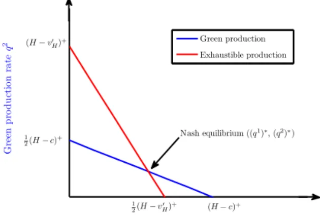
2.1 Nash equilibrium of the Cournot duopoly in high-demand regime. The two piecewise linear curves show optimal production rates of player 1 and player 2 given v0_H(x) and the production rate of the other player (e.g. q1,∗₍_x_;_q2₍_x₎_{, v}0

H(x))) as defined in (2.7). Equilibrium is achieved

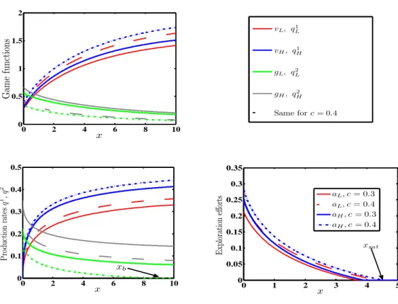
when the curves cross. . . 40 2.2 Duopoly axis game solutions for two different levels of production cost c: solid curves are for c= 0.3; dashed for c= 0.4. Tope left panel: Game functions vi(x), gi(x). Bottom left panel: Production rates qi`(x), ` = 1,2. Bottom right panel: Exploration efforts ai(x) of exhaustible

producer 1. We take linear inverse demand with L = 0.75, H = 1, and switching rates λ01 = 1₃, λ10 = 1₅. Exploration costs are Ca(a) =

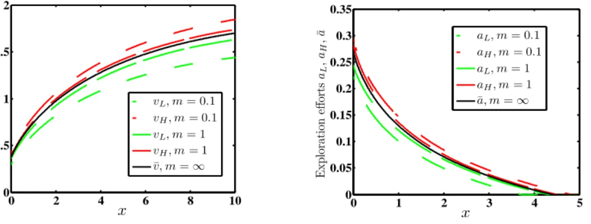
0.1a+a2/2. . . 47 2.3 Left panel: convergence of the game functions vi(x) → v¯(x) as λ01, λ10 → ∞ together. Right panel: convergence of the exploration effort ai(x)→a¯(x). We take λ01 =m/3, λ10 =m/5, with m = 0.1,1 as well as the limiting solution defined in Lemma 2.2. . . 52 2.4 Left panel: xstart as a function of λ01 ∈ [1/3,3]. Middle panel: xstart as a function of H ∈ [L,1.5]. Right panel: xstart as a function

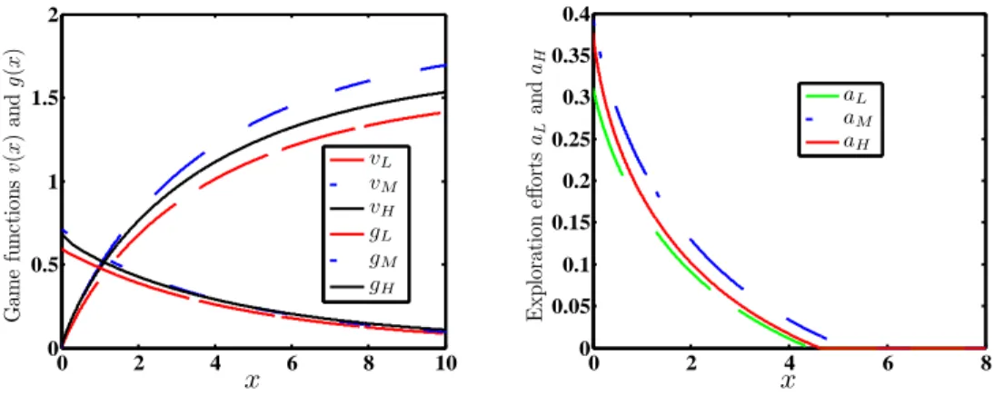
of green production cost c _∈ [0, H]. The default parameters are L = 0.5, H = 1, c= 0.3, λ01= 1₃, λ10= 1₅. . . 54 2.5 Duopoly with three demand regimes, D1 = L, D2 = M, D3 = H. Left panel: Game functions vi(x) and gi(x), i = L, M, H of the two

producers. Right panel: exploration efforts ai(x),i=L, M, H. We take L= 0.5, M = 1, H = 1.5 andλ12= 1₂, λ23= 1₄, λ31= 1 in (2.23). . . 58

(16)

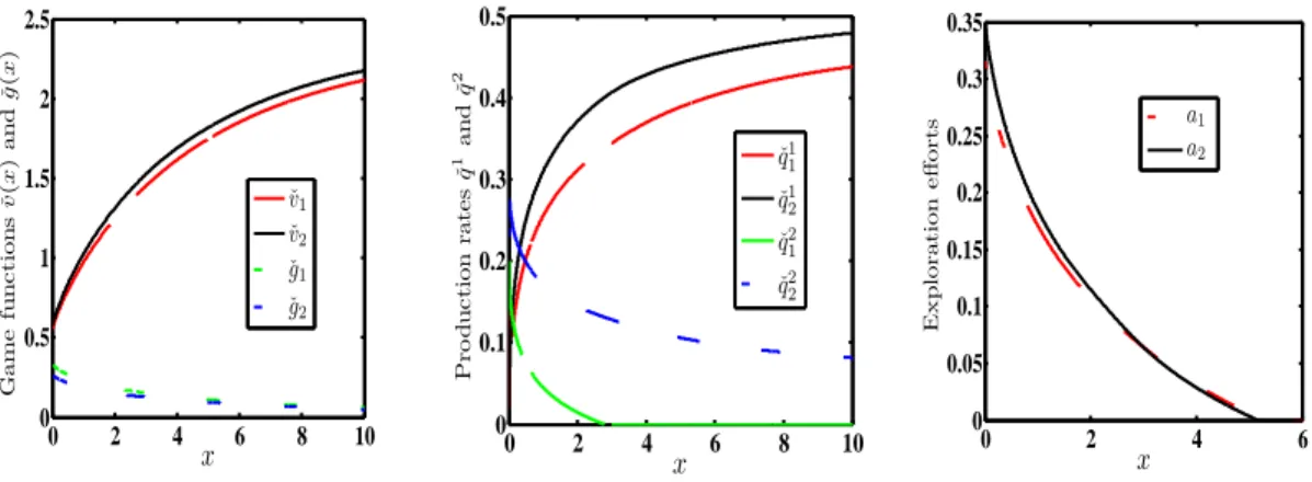
2.6 Duopoly with regime-switching green production costs. Left panel: Game functions ˇvi(x) and ˇgi(x), i = 1,2 of the two producers. Middle

panel: Production ratesq_i`(x) of the two producers`= 1,2. Right pane: Exploration efforts ai(x) of the exhaustible producer. We take ¯D =

1, c1 = 0.4, c2 = 0.6, and switching rates λ01 = 1₃, λ10 = 1₅. Exploration costs are Ca(a) = 0.1a+a2/2. . . 61

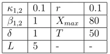
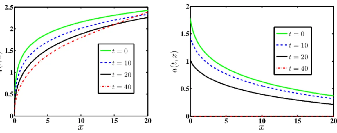
3.1 Production and exploration controls (q, a) associated with the HJB equation (3.8) under constant pricep(t) = 3 andλ(t) = (1₋0.025t)+_,₀_≤ t _≤ T. Left panel: production rate q(t, x). Right panel: optimized ex-ploration rate a(t, x). . . 86 3.2 Evolution of reserves distribution under the production and ex-ploration controls (q, a) obtained in Section 3.3.1. The discovery rate is

λ(t) = (1₋0.025t)+_{and unit amount of a discovery is}_δ_{= 1. Left panel:} Density of reserves distribution m(t, x) = ₋_∂x∂ η(t, x) for several t’s. Right panel: Proportion of producers with no reserves π(t) = _P(Xt = 0). 89

3.3 Convergence of the numerical scheme in Section 3.3.3. We start with initial guess p(0)₍_t_{) = 3}_∀_t _∈ _[0_{, T}_{], and discovery rate} _λ₍_t_{) = (1}₋ 0.025t)+. Game value functionv(k)(t, x) converge after k_≥4 iterations, with t = 10 fixed. . . 92 3.4 Evolution of total production Q(t), total reserves R(t), and total discovery rate A(t) as a function of t. We compare exploration with discovery rateλ(t) = (1₋0.025t)+_{, in comparison to zero discovery rate} λ(t) = 0. . . 94 3.5 Evolution of reserves distribution with exploration λ(t) = (1 ₋ 0.025t)+_{, in comparison with no-exploration} _λ₍_t_{) = 0. Left Panel:} Pro-portion π(t) of producers with no reserves at time t. Right panel: Pro-portion η(t, x) of players at time t with reserves level greater than x. . 94 4.1 MFG solution with a constant λ(t) _≡ λ = 1 to illustrate the re-lationship between the time-dependent and stationary solutions. Upper left panel: Densitym(t, x) of reserves distribution. Upper right: Propor-tion π(t) of producers without reserves. Lower left: Total exploration rate A(t) and total production Q(t). Lower right: Total reservesR(t). 101 4.2 Stationary MFG solution as a function of discovery rate λ. Left panel: Total production ˜Q. Middle: Stationary reserves ˜R; Right: Sta-tionary proportion ˜P of producers with no reserves. . . 103 4.3 Effect of discovery rateλon exploration effort. Left panel: Station-ary exploration effort ˜a(x) with different values of λ. Right: Stationary saturation level ˜xsat = inf{x≥0 : ˜a(x) = 0} as a function ofλ. . . 104

(17)

4.4 Effect of discovery rateλon reserves distribution. Left panel: Den-sity ˜m(x) of stationary reserves distribution with different values of λ. Right: Standard deviation Stdev( ˜X) of stationary reserves distribution against discovery rateλ, whereStdev( ˜X) =

q −R0∞x 2_η_˜₍_dx₎_{− −}R∞ 0 xη˜(dx) 2 . 105

4.5 Equilibrium production and reserves level in the regime λ =λ/

and δ = δ for different values of . Left panel: Evolution of total

production Q(t). Middle: Stationary production ˜Q against . Right :

(18)

Chapter 1 Introduction

We study production and exploration of exhaustible resources for the purpose of generating energy. Exhaustible resources, such as oil, coal, and ores have great importance in the functioning of the whole economic system. Dwindling oil re-serves and the resulting impact on energy supply and price is of fundamental importance to the functioning of the whole economic system. Energy production with the resources generates revenue but lowers remaining reserves for further production. Exploration for new resources will likely lead to discoveries that add to reserves for production, though exploration is costly and discoveries occur in an uncertain way. In oil industry, for instance, exploration activities include re-search and development of new drilling techniques, and putting human labors and facilities into scanning geographic areas for new resources.

(19)

Exploration is one of the main interests in the research. Mathematically we use a point process to model the exploration. Jumps of the point process mark the discovery times. The amount of each discovery can be random in general, but we assume it is a constant positive quantity without loss of any generality. The intensity of the point process is subject to the control of producers. More effort input leads to higher frequency of new discoveries as well as higher exploration costs.

Energy markets can be viewed as companies competing with each other in energy production and exploration for new resources, for the purpose of profit maximization. Each energy company is regarded as a producer. It is of great interest to study the competition between the energy producers and the resulting equilibrium prices and total supplies. Due to the competitive nature of energy markets, game theory is a useful tool to study the outcome of the competition. Game theory deals with strategical interactions among multiple decision makers, who are also called game players in game theoretic language. Each player has an objective function and chooses strategic variables to optimize the objective function. The strategic variables are also called controls from the perspective of optimization. The players interact with the others in the way that each one’s ob-jective function involves the strategic variables of the others, thus one has to make decision by taking into account the strategies of the others. Producers in energy

(20)

markets can be viewed as players competing with each other in order to maximize profit. The strategic variables of players in the research are production quantity and exploration effort. We work in a Cournot game framework in which players choose quantities of energy production and receive profit based on a single market price determined through aggregate supplies. In contrast to the Cournot game, where the strategic variable is quantity of production, the other type is Bertrand game, in which price is the strategic variable of the players. Harris, Howison, and Sircar [31] studied Cournot model of exhaustible resources, while Ledvina and Sircar [39] studied Bertrand model. The game we study is non-cooperative, since producers make decisions independently without any cooperation.

The players competing with each other by choosing strategies of production and exploration, in order to maximize expected profit. The game equilibrium of our interest is Nash equilibrium, which is a set of all players’ strategies such that no one can better off by unilaterally changing individual strategy. A single player’s decision depends on the reserves levels of all players, thus the controls take the feedback form. Moreover, the control variables are Markovian, that is, the decisions are based on current reserves level that contains sufficient informa-tion of the past. Since the players choose strategies from the admissible set of Markov feedback controls, the game equilibrium we study is Markov feedback Nash equilibrium.

(21)

Due to the game nature and stochasticity, the research is embedded in the framework of stochastic differential game. Stochastic differential game is closely related to stochastic control theory. Isaacs [35] is a good reference for introduc-tory differential game. We mention [24] as a reference for stochastic control and stochastic differential game. The basic formulation of stochastic control involves a dynamic system driven by stochastic factors, whose state evolution can be influ-enced by exercising controls. Associated with the system is an objective function which depends on the state process and controls over either a finite or an infinite time horizon. The main goal is to find the control that can achieve the optimal (minimal or maximal) value of the objective function. The objective function un-der the optimal control is called value function. Dynamic programming method is employed to solve for optimal control, which equates the value function under optimal control to the value realized in a local infinitesimal time interval under optimal control plus the value function after that. By dynamic programming method, we obtain a partial differential equation of the value function in terms of time and state variables, which is formally calledHamilton-Jacobi-Bellman (HJB) equation. Optimal control is linked to the value function through the HJB equa-tion. thus we can solve for optimal control by solving the equaequa-tion. In stochastic differential games there are players associated with a stochastic dynamic system, on which they can exercise controls. Each player has an objective function

(22)

de-pending on the state variable of the stochastic dynamic system and the controls. All the players are interrelated in such a way that each player’s value function in-volves other players’ state variable and controls as well as his own. The controls in the game theoretic context are also calledstrategies. Each player has to consider all the other players’ strategies while making his own strategy. Since the objective function value each player achieves is though game, we call it game value func-tion. We use dynamic programming method to solve for the equilibrium strategies. Since each player’s game value function involves other players’ controls, we need to freeze other players’ controls when we derive the partial differential equation for one player. The system of partial differential equations of game value functions is calledHamilton-Jacobi-Bellman-Isaacs (HJB-I) equations. HJB-I equation is a main tool we use to solve for Nash equilibrium strategies in the research.

The research is organized as follows. In Chapter 2, we study Cournot game between two producers of different resource types under stochastic demand. Par-ticularly we study how stochastic demand affects the Nash equilibria of the game. In Chapter 3, we employ mean field game approach to find approximate Markov Nash equilibrium of Cournot game with a continuum of exhaustible producers. Numerical schemes are developed to solve the resulting system of partial differen-tial equations. In Chapter 4 we study a time-stationary mean field game model, in which the reserves level remains invariant due to the counteracting effects of

(23)

production and exploration. We also study the effect of randomness of exploration process on equilibrium production and reserves distribution.

In Chapter 2 we study a game model between two energy producers of dif-ferent resources: producer 1 that extracts an exhaustible resource (oil) and has to worry about diminishing reserves; and producer 2 that extracts a renewable resource (green energy such as solar power) and therefore has infinite reserves. Two stochastic state variables are considered: current reserves level of the ex-haustible player 1 and demand level. Moreover, players have a total of three controls, namely productions rates for players 1 and 2, as well as exploration ef-fort for producer 1. The exhaustible reserves level follows piecewise deterministic trajectories, smoothly decreasing due to production and experiencing constant-size jumps upon new reserves discovery. These upward jumps of fixed constant-size mimic discrete discoveries of new oil fields or new oil recovery technologies that take place abruptly. The demand level is modeled as a continuous-time Markov chain that switches among different regimes to mimic business cycle fluctuations.

The two producers in Chapter 2 compete through a Cournot framework, in which producers choose quantity of production and receive profit based on a single market price determined through aggregate supply. Costs of the exhaustible player are driven solely by the costly (convex) exploration effort; her production costs are taken to be zero. On the contrary, the green producer has a positive marginal

(24)

cost of production but inexhaustible resources. These production costs of player 2 are a proxy for the amount of competition. They also reflect the present reality of non-renewable energy production as being the cheaper incumbent against the new renewable entrants. The Cournot framework is used because at the macro level, energy is perfectly substitutable and so the two producers’ products are in direct competition. Producers’ profits are equal to the quantities of production multiplied by the market price, minus the cost of exploration (player 1) or produc-tion (player 2). The game value funcproduc-tions of the two players are the discounted cumulative expected profits starting with certain initial reserves level and demand regimes.

The aim of Chapter 2 is to study the game between the exhaustible pro-ducer and the green propro-ducer in terms of dynamic Nash equilibria, and partic-ularly the impact of stochastic demand on the game equilibria. The model is cast in continuous-time so as to allow use of the Hamilton-Jacobi-Bellman-Isaacs methodology that reduces computational analysis to study of coupled systems of differential equations. We use dynamic programming method to obtain a system of HJB-I equations of the players’ game value functions. Those equations are first-order nonlinear forward-delayed ordinary differential equations. The equations are first-order due to the lack of diffusive stochastic factors such as Brownian motion. The forward-delay term is due to the controlled point process that marks the

(25)

mo-ment of new discovery. Moreover since only a single agent has reserves, there is just one continuous state-variable, effectively allowing us to deal only with ordi-nary differential equations rather than partial differential equations. Particularly the equilibrium production of the two players are piecewise-linear in the derivative of game functions, which leads to piecewise-defined with free boundaries between adjacent pieces. Towards the end of chapter 2 we also mention some extension of the Cournot model by considering stochastic cost of renewable energy production. In chapters 3 and 4, we study Cournot game with a continuum of homogeneous exhaustible producers. Each producer has production quantity and exploration effort as control variables. The single market price is determined by all produc-ers’ total production. Both production and exploration are assumed to be costly. Each player has game value function that equals to the discounted amount of profit minus costs, where the profit and costs are realized under the equilibrium strategies of all players. We aim to study equilibrium production quantities and reserves distribution in energy markets with a large population of competing pro-ducers. Particularly, we want to understand how exploration activities affect the long-term market organization, and how the exploration uncertainty permeates the solution.

According to the classical HJB-I method for an N-player game, each player is associated with an HJB-I equaiton and thus the model involves a system of N

(26)

partial differential equations which is intractable. We employ mean field game approach to model energy markets with a continuum of exhaustible producers. The mean field game model reduces the system ofN partial differential equations to a system of two doubly coupled partial differential equations: one is the HJB equation of a representative player’s game value function; and the other is the transport equation of all players’ reserve distribution. The market price, directly related to the total production of all the producers, enters the game value function of the representative producer as the mean field term. The representative player chooses his optimal quantity of production and exploration effort depending on all the other players strategies through the mean field term market price.

1.1 Games with Exhaustible Resources

It is worthwhile mentioning models of single-agent before considering games with more than one agents. There is a long literature on optimal economic behavior of a natural resource monopolist extracting non-renewable resources. Hotelling [32] found that without discovery exhaustible resource price grows at inter-temporal discount rate. Pindyck [44] studied a deterministic model of ex-ploration for exhaustible resources. In the model exex-ploration was assumed to be incremental and represented as a deterministic reserve addition. It was shown that the resulting resource shadow price, corresponding to the marginal value of

(27)

additional reserves will firstly decrease and then increase as reserves run low. As extensions to Pindyck [44] there is a series of works studying exploration. Arrow et al. [2, 21, 30, 47] represented exploration, which is punctuated by large discov-eries, as a point process. Pindyck [45] further studied a model in which the total size of reserves is unknown. The dynamics was then described via a stochastic differential equation with controlled volatility and drift. Dasgupta and Heal [19] is a comprehensive reference for literature on exhaustible resources up through the 1970s.

The first paper that rigorously treated a dynamic non-cooperative model for exhaustible resource extraction was published by Harris, Howison, and Sircar [31]. They studiedN-player continuous-time Cournot game in which firms choose pro-duction quantities. The games were characterized by a system of nonlinear HJB partial differential equations which were analytically and numerically hard to re-solve. They also analyzed the problem when there is an alternative, but expensive, technology (for example solar power for energy production). They illustrated the two-player problem by numerical solutions, and discussed the impact of limited oil reserves on production and oil prices in the case of two-player model.

Ludkovski and Sircar [40] studied a related model that allowed for stochastic evolution of reserves by considering exploration that can lead to discovery of new reserves. This analysis was motivated by the oil market where E&P (exploration

(28)

and production) efforts total many billions of dollars a year. In that sense, while oil is exhaustible, it is also replenishable since there is a difference between total abstract reserves on Earth, and what is actually commercially “proven” and drives production decisions. With exploration, players have two complementary choices regarding running down existing reserves and expending effort in the hopes of finding new reserves. In particular, players may never fully “leave” the game since they can periodically resurrect themselves by ongoing discoveries. In [40], they firstly treated the case of a monopolist who produces and may undertake costly exploration to replenish his diminishing reserves. Then a stochastic game between an exhaustible producer and a “green” producer was studied. The new discoveries were modeled through a controlled jump process with intensity given by exploration efforts. The game between the two players led to a study of systems of non-linear first-order delay ordinary differential equations with implicit boundary conditions. The delay term and implicit boundary conditions were due to the nature of jumps in the model.

In my work [41] Dynamic Cournot Models for Production of Exhaustible Com-modities under Stochastic Demand, which is the main content of Chapter 2, I extended the work [40] by studying the effects of stochastic demand on the equi-librium of the dynamic Cournot game between an exhaustible resources producer and a renewable resources producer. The state variable is the reserves level of

(29)

exhaustible resources, which decreases at a (controlled) production rate and in-creases through a random process that has discrete increment at a controlled rate (this process is formally called controlled point process). The market price is a negative function of the aggregate production of the two producers. The game function of exhaustible producer is the total discounted profit over infinite time horizon that is determined by the total revenue(product of price and production) minus the exploration cost. The game function of renewable producer is the total revenue minus production cost. The game functions of the two players are coupled through the market price which is a negative function of their total quantity of production.

We considered stochastic demand as a simulation of macroeconomic volatility. The exogenous stochastic demand factor is modeled through a continuous-time Markov chain that switches between high and low regimes(it can be generalized to a process such as an Itˆo diffusion, but two-regime setting is sufficient to represent the market demand ups-and-downs volatility). The Markov chain enters the linear price function as a coefficient that moves the price between high and low regimes. We studied how the demand regime changes affect game equilibria, and compared with the case of deterministic demand in [40].

Due to demand regimes switching, each player is associated with one game function in each regime, which leads to a total of four game functions for two

(30)

players in two regimes. In infinite time horizon, the model is time stationary. Thus the HJB-I partial differential equations become HJB-I ordinary differential equation, with time-derivative term vanishing. Due to the random discrete in-crement term in the dynamics of the state variable, the HJB-I equations involve forward-delay terms and implicit boundary conditions. The optimal control of the two players depends on the value function of the exhaustible producer, thus the HJB-I ordinary differential equations of the exhaustible producer is autonomous of those of the renewable producer. It is sufficient to analyze the HJB-I ordi-nary differential of the exhaustible producer to obtain the equilibrium production strategies of the two players.

The major challenge is that the function forms of the HJB-I ordinary dif-ferential equations are piecewise-defined with free boundaries between each two adjacent pieces. The free boundaries occur because the optimal controls of the two players are piecewise linear in the derivative of the game function of exhaustible producer. The interaction of the forward-delay term and the piecewise-defined functional form of ordinary differential equation poses a challenge. To the best of our knowledge, there is no reference about well-posedness of such equations. But using numeric method we solve an approximation to the system of equations that is guaranteed to be well-posed. To deal with the forward-delay term in the equa-tions, we use an iterative scheme that starts without the delay term, and iteration

(31)

goes on by taking the data from the last iteration to substitute the forward-delay term. In each iteration, we use fourth-order Runge-Kutta scheme to solve for the system of ordinary differential equations. This iterative scheme was proved to be convergent both analytically and numerically, according to [40].

Due to stochastic demand, the game equilibria become more complicated than the deterministic demand model in Ludkovski and Sircar [40]. A novel finding in the research is a new possible game equilibrium due to the stochastic demand. In the low regime, it is possible that the exhaustible production shuts down thus the renewable producer monopolizes the market. Exhaustible production shuts down for two reasons: one reason is the difference between high and low demand regimes is large thus it is profitable to shut down production in low regime in order to save reserves for production in high regime; the other reason is that the average holding time in low regime is short enough thus extra profit made in high regime can compensate the loss in low regime due to production shutdown. Production shutdown also leads to extra mathematical difficulty, because in this situation the derivative of game function zeros out, the ordinary differential equation in the low regime degenerates into an algebraic equation. In computation we have to detect when this happens, and then we need to switch to a new ordinary differential equation derived from the algebraic equation.

(32)

Since the stochastic demand is a simulation of macroeconomic volatility in the research, it is interesting to study how the game equilibrium changes as the frequency of regime switching changes. We use the asymptotic expansion of the game functions in terms of the average holding times in the two regimes, and by letting the average holding times in both the two regimes goes to zero we obtain the ordinary differential equation for limiting game function, which is again a piecewise-defined ordinary differential equation with forward-delay term and im-plicit boundary condition. By numerically solving the ordinary differential equa-tion we obtain the equilibrium producequa-tion and exploraequa-tion when market demand volatility is high.

The single-agent and two-player models [40, 41] will be extended to a model with a continuum of players [42], which is introduced in Chapters 3 and 4. We employ mean field game approach to find approximate Nash equilibrium of the game, which will be introduced in the following Section 1.2.

1.2 Mean Field Game Approach

The second part of the research studies energy market with a continuum of producers. Mean field games (MFG) approach is applied to model the strate-gic interactions among a continuum of players and the resulting equilibrium of production, exploration, and distribution of resources reserves. In a differential

(33)

game model with a finite number N of players, their equilibrium strategies can be determined by a system of Hamilton-Jacobi-Bellman-Isaacs (HJB-I) equations derived from the dynamic programming principle. The dimension of the system in general increases as the numberN of players increases, which makes the game model intractable for large N. Mean field game (MFG) approach simplifies the modeling by considering equilibria with a continuum of homogenous players; the respective finite dimensional game state translated into a measure η. The main idea is to consider an optimization problem of the representative agent; the latter becomes a regular stochastic control problem with the competitive effect captured via a certain aggregate mean-field interaction driven byη. In turn, the aggregate behavior of the players implies dynamics on the distributionηof agent states. This leads to a system of two infinite-dimensional partial differential equations (PDEs) which is viewed as an approximation to the N-system of finite-dimensional PDEs in the original finite-N setup.

The MFG framework was introduced by Lasry and Lions [36, 37, 38] and Caines, Huang, and Malhame [34]. A formal introduction to the basics of mean field games and mean field type control can be found in Bensoussan, Frehse, and Yam [3]. Cardaliaguet [6] studied a system of first order mean field game equations with local coupling in the deterministic limit. A system of (possibly degenerate) second order mean field game partial differential equations was analyzed in [7], and

(34)

existence and uniqueness of suitably defined weak solutions were proved. Carmona and Delarue [13] provided a probabilistic analysis of a large class of stochastic differential games for which the interaction between the players is of mean-field type, and proved that solution of mean field game indeed provides approximate Nash equilibria for games with a large number of players. Bensoussan, Sun, Yam, and Yung [4] provided a comprehensive study of a general class of linear-quadratic mean field games. Mean field games between a major player and a continuum of minor player can be found in [33, 43, 15]. Mean field game models with local coupling can be found in [5, 6, 7]. Cardaliaguet, Lasry, Lions, and Porretta [8] studied a locally coupled mean field game model defined on a finite time horizon and showed that the system converges to a stationary mean field game as time horizon tends to infinity. It was studied in [9] that a mean field game model with nonlocal coupling on a finite time horizon converges exponentially to the associated stationary mean field game model, a time horizon tends to infinity.

Achdou, Camilli, and Capuzzo-Dolcetta [1] introduced finite difference schemes for stationary and evolutive mean field game models, and proved convergence of the numerical schemes under various assumptions on the coupling operator. Carlini [10, 11] proposed fully discrete semi-Lagrange schemes for mean field game systems of first order and second order, and proved convergence of the numerical schemes. In [29, 16, 17], iterative schemes were used to solve the coupled mean

(35)

field game partial differential equations associated with dynamic Cournot models for production of exhaustible resources.

The mathematical significance of the MFG approach is that it provides a tool to study (differential) games with a large population of players. Specifically, the MFG setup leads to an HJB equation to model a representative player’s strategy, and a transport equation to model the evolution of the distribution of all the play-ers’ states. In our context, the states are the reserves’ levels, and the interaction is via the market pricepthat is related to total production across all the producers. Thus,penters the game value function of the representative producer as the mean field term and drives his optimal quantity of production and exploration efforts conditional on the other producers’ strategies. In turn, the distribution of reserves is driven by the latter production rates and exploration efforts.

The study of exhaustible resources oligopolies using MFGs was initiated in Gu´eant et al. [28, 29] who studied a mean field Cournot model with a linear-quadratic production cost function, and a stochastically fluctuating reserves pro-cess. They further introduced generalized models that consider value function depending on further factors, e.g. they included a ranking effect into the value function. They also considered competition between producers of two types of resources. Graber [25] introduced a linear quadratic mean field game model of exhaustible resource production, in which the reserves process of a representative

(36)

player is influenced by a common noise with all other players, as well as its individ-ual noise. [25] at the beginning studied a general linear quadratic mean field type control problem by giving solution both in terms of a forward/backward system of stochastic differential equations and by a pair of Riccati equations. [25] further gave certain conditions so that the mean field type control problem is equivalent to a class of mean field game problems. [25] then gave a model of exhaustible resource production, and connected it to an equivalent linear quadratic mean field type control problem. By solving the associated pair of Reccati equations, equilibrium production and market price are obtained in explicit form.

Chan and Sircar [16, 17] showed that the mean-field equilibrium for production of exhaustible resources is the same for both Bertrand and Cournot type compe-tition. Cournot competitions between exhaustible and renewable resources were studied in [17]. They first considered competition of producers, each of whom can produce costly renewable resources once exhaustible reserves run out. Then they studied competition of a large group of exhaustible producers with a single renew-able producer, similar to the major-minor model of Huang [33]. It was found that when renewable production cost is high, the exhaustible producers may strategi-cally increase production rate and hence lower the price. They also studied the impact of exploration and discovery in Cournot models of exhaustible resources and found that higher reserves lower exploration rates and increase production.

(37)

We apply the MFG approach to model energy markets with a continuum of producers of exhaustible resources. Through the mean field formulation, we aim to study equilibrium production quantities and reserves distribution in energy markets with a large population of competing producers. Particularly, we want to understand how exploration activities affect the long-term market organiza-tion, and how the exploration uncertainty permeates the solution. Three main quantities that we wish to investigate are: (i) the price effect of exploration, and related time-evolution; (ii) aggregate production implied by the model; (iii) ag-gregate exploration efforts. The related analysis yields quantitative insights into the macro behavior of major commodity markets, especially those for fossil fuels (crude oil, natural gas) where exhaustibility and associated E&P (Exploration and Production) activities are key to strategic behavior of the firms.

In comparison to previous studies and MFG models, our setup has several key differences. First, the price interaction coming from the aggregate production rate yields a non-standard mean-field coupling between the agentcontrols (rather than the more common state-space interaction), necessitating special treatment in the HJB equation. Second, the jump process modeling discrete reserves discoveries leads to a integral term in the HJB equation and a non-local term in the transport equation. Third, the hard constraint of exhaustibility (i.e. zero reserves) generates

(38)

a non-standard, implicit boundary condition at x = 0 which again requires a tailored solution.

Our work fits into two different strands of game-theoretic models of energy production. On the one hand, we extend the works [16, 29] who considered ex-haustible resources but without exploration; thus reserves were non-increasing. Specifically, the reserves processes in [29, 16] are modeled by Itˆo diffusion pro-cesses, and the transport equation of reserves distribution is determined by a standard Kolmogorov forward equation. In contra-distinction, in this chapter we consider exploration activities that stochastically lead to additional reserves. Thus, the reserves process is a controlled jump process generating a non-local, first-order transport equation. On the other hand, we extend the duopoly model [40]. In the latter model of an exhaustible producer and a renewable producer, each one has significant power of influence on price; in the MFG model herein, each producer has negligible power on market price that is rather driven by the

aggregate production.

The closest work to ours is Chan and Sircar [17] who also considered an MFG setting with exploration. We give a more comprehensive investigation of explo-ration effects on game equilibrium in terms of total production, reserves distribu-tion, and producers’ behavior in limiting situations of exploration and discovery.

(39)

The above features generate several major challenges. For example, due to the jump process, the transport equation of the reserves distribution in our research

is a partial integro-differential equation which leads to some more analytical and

numerical difficulty. A major part of the paper is devoted to constructing an iterative numerical scheme to solve the MFG equations. Our numerical scheme decouples the HJB and transport equations via a Picard-like iteration that alter-nately updates the optimal production and exploration controls, and the reserves distribution function (which in turn determines the market price). Furthermore, since the HJB equation depends on time and space, we use method of lines to solve the HJB equation, that is, we discretize the HJB equation in the space di-mension but not in time and solve the system of ordinary differential equations using fourth-order Runge Kutta method.

1.3 Model

1.3.1 Reserves Process

We consider a game model with N exhaustible producers (players). Each producer uses exhaustible resources, such as oil, to produce energy. Let X_ti rep-resents the reserves level of player i, i = 1, ..., N. Each Xi

t belongs to the state

(40)

controlled production rateqi

t≥0, and increases by jumps due to discovery of new

resources. We use a controlled point process to model occurrences of new discov-eries. Specifically, occurrences of new discoveries for playeriare modeled through a point process Ni

t with controlled intensity λ(t)ait, where ait is the exploration

efforts controlled by the player andλ(t) is rate of discoveries per unit exploration effort. The parameter λ(t) reflects the current exploration techniques and overall resources underground, hence it is taken as externally given and uniform for all producers. Since the total resources underground is decreasing due to exploration and production, it is reasonable to assume that λ(t) is decreasing in time and

lim

t→∞λ(t) = 0.

Let τ_ni be the n-th arrival time of the point process N_ti, then the inter-arrival time between the n-th and (n+ 1)-th arrivals satisfies the following probability distribution P τ_ni₊₁ > τ_ni +t= exp − Z t 0 λ(s)ai_τi n+sds . (1.1)

The positive quantityδ is the unit amount of a discovery, which is assumed to be constant as in [40, 41]. The unit amount δ of each discovery can be random in general, which we will address in the context of specific optimization problems. These upward jumps of fixed size δmimic discrete discoveries of new oil fields (or perhaps new oil recovery technologies) that take place abruptly. Such

(41)

“Poisso-nian” dynamics date back to work of Arrow and Chang [2] and are arguably more fidel to realistic reserves evolution. According to the setups above, the reserves dynamics of the players are given by the following stochastic differential equations

dX_ti =₋qi_t1{Xi

t>0}dt+δdN

i

t, t >0, (1.2)

X₀i =xi₀ _≥0, i= 1,2, ..., N.

where each playeriis assumed to have initial reserves levelxi₀,i= 1,2, ..., N. The indicator function ₁{Xi

t>0} implies that production shuts down whenever reserves run out, i.e., Xi

t = 0. The N players’ reserves can be represented by a random

vector defined as

XN_t := X_t1,_{· · ·} , X_tN.

The controlled dynamics (1.2) of the reserves can be described as piecewise

deter-ministic process (PDP), because between discoveries no new information is coming

in and reserves decrease continuously according to the production schedule. At discovery moments, reserves increase via an instantaneous jump of sizeδ.

1.3.2 Cost Functions

We assume that all producers have the same cost functions of production and exploration, denoted by Cq(·) and Ca(·), respectively,

Cq(q) =κ1q+β1 q2

2, Ca(a) = κ2a+β2

a2

(42)

The coefficientsβ1,2of the quadratic terms are assumed to be positive, which make the cost functions strictly convex forq and a large enough. Convexity of the cost functions guarantees that the optimal production and exploration effort levels are finite. The coefficients κ1,2 of the linear terms represent constant marginal cost of production and exploration arisen from the use of facilities and labor. The coefficients β1,2 of the quadratic terms represent increasing marginal cost proportional to quantities of production and exploration efforts. Production and exploration of exhaustible resources lead to negative externalities (such as rising labor costs or nonlinear taxation). We note that when κ2 = 0 then exploration is ongoing, otherwisea∗ = 0 could be optimal.

1.3.3 Price Determination

The market price pis determined from the global supply-demand equilibrium. The total demand is determined through a demand function p _→ D(p) which gives total demand levels at each price level p. The producers sell total quantities

Q into the market and receive price p determined through a price function p(Q). In the global supply-demand equilibrium, the price function should be equal to the inverse demand function D−1₍_Q_{), i.e.} _p₍_Q_{) =} _D−1₍_Q_{). We assume a linear}

(43)

price (or inverse demand) function

p=p(Q) = ¯D₋Q, (1.4)

where Q := PN_i₌₁qi _{is the total production of all} _N _{producers, and ¯}_D _{is the}

maximum (finite) choke price under zero supply. Producers interact with each other through this price mechanism that is driven by the aggregate supply (and affects player’s profits) leading to non-cooperative game.

1.3.4 Game Value Functions and Strategies

In a continuous-time Cournot game model, each player chooses rate of pro-duction qi _{in order to maximize profit which is equal to the revenue} _p_·_qi_{, minus}

the production and exploration costs, integrated and discounted at a rate r >0. We work on a finite time horizon [0, T], where T is exogenously specified. The role of the horizon will be revisited in the sequel. The price each player receives is determined through the inverse demand function (1.4).

We define the strategy profile sof all the N players by

s:= s1, s2, ..., sN,

with each player i’s strategy vector denoted by si _{:= (}_qi_{, a}i_{). Starting with initial}

(44)

is defined as the total discounted profit Ji₍_s_;_t,_x_{) :=} E (Z T t " D−1 N X j=1 qj_s ! qi_s₋Cq(qsi)−Ca(ais) # e−r(s−t) ds Xt=x ) , (1.5) where the expectation is over the random point processes Nj _{that drive} _Xj _and

hence qj’s. Associated with the objective functional, we define player’s i best response value function conditional on other players’ strategies _{sj,∗

}j6=i as the supremum vi(t,x) := sup si_∈AJ i s1,∗, . . . , si−1,∗, si, si+1,∗, . . . , sN,∗;t,x, i= 1, . . . , N. (1.6)

We focus on the admissible set_Aof strategies wherebysi_t= (qi_t, ai_t) are Markovian feedback controlsqi

t =qi(t,Xt),ait=ai(t,Xt) such thatJi(s;t,x)<∞,∀x∈RN+, for all i = 1, . . . , N. The exhaustibility constraint also imposes that qi(t,0) _≡ 0 is the only admissible control.

From (1.5) and (1.6), we see that each player’s choice of strategy depends on the strategies of all the others. We aim to study the Nash equilibrium of this game. To be more precise, we look for Markov feedback Nash equilibrium, because the strategies set from which the players choose is of Markov feedback form.

Definition 1.1 (Nash equilibrium of N-player game). The Nash equilibrium of

(45)

si,∗ _{= (}_qi,∗_{, a}i,∗₎ _{such that}

Ji₍_s∗

;t,x)_{≥ J}i (s∗,−i, si);t,x, _∀i_{∈ {}1,2, . . . , N_}, (1.7)

where s∗,−i _{is the strategy profile} _s∗ _{with the} _i_{-th entry} _si,∗ _{replaced by arbitrary}

si = (qi, ai)_{∈ A}.

In words, a Nash equilibrium is the set of strategies of the N players such that no one can better off by unilaterally changing his own strategy. The feedback structure of the controls qi_t =qi(t,Xt), ait = ai(t,Xt) together with (1.4) imply

that playeri’s dependence onXt can be summarized by his individual reservesXti

and the aggregate distribution of all players’ reserves. The latter is characterized through the upper-cumulative distribution function defined by

ηN(t, x) := 1 N N X j=1 1_{X_tj≥x}. (1.8)

Thus the Markovian feedback controls (qi, ai) can be equivalently represented as

q_ti =qi t, X_ti;ηN(t,_·), a_ti =ai t, X_ti;ηN(t,_·), i= 1, . . . , N. (1.9)

Theoretically the Nash equilibrium of the N-player game can be found by Hamilton-Jacobi-Isaacs (HJB-I) approach. HJB-I approach is to use dynamic programming principle to derive the partial differential equation of each player’s game value function, with other players’ strategies as entries. It is extremely hard to find a Nash equilibrium by using the (HJB-I) approach either analytically or

(46)

numerically, even for small N, e.g. N = 2. In Chapter 2 we study the Cournot game between an exhaustible producer and a renewable producer in high and low demand regimes, which involves a system of equations with dimensionality equal to two (number of players) by two (number of demand regimes). The re-newable producer has infinite resources, but has positive fixed production costs. The production strategy of the renewable producer depends on the production of the exhaustible producer. Only the exhaustible producer has controls on the reserves level as the unique state variable. Hence the equations of the exhaustible producer are autonomous from the equations of the renewable producer, and it suffices to deal with the equations of the exhaustible producer to obtain the Nash equilibrium of the game. Moreover, We consider the stationary case in which exploration can go forever, thus we just need to deal with a system of ordinary differential equations.

In Chapters 3 and 4, we employ mean filed game approach to find approximate Nash equilibrium of Cournot game involving a continuum of players (N _{→ ∞}), which reduces the system of N coupled equations in HJB-I framework to two doubly coupled equations: one is the HJB equation of a representative player; and the other is the equation of the evolution of distribution of all the players.

(47)

Chapter 2 Dynamic Cournot Game Under

Stochastic Demand

2.1 Model Overview

In this chapter we study dynamic Cournot games between two players: pro-ducer 1 that extracts a non-renewable resource (oil) and has to worry about re-serves; and producer 2 who extracts a renewable resource (green energy) and therefore has infinite reserves. We also consider two stochastic state variables: demand Dtand current reserves Xtof the exhaustible player 1. Moreover, agents

have a total of three controls, namely production rates for producers 1 and 2, as well as exploration effort for producer 1.

(48)

The two producers compete through a Cournot framework, in which producers choose quantities of energy to produce and receive profit based on a single market price determined through aggregate supply. Costs of the exhaustible player are driven solely by the costly (convex) exploration efforts; her production costs are taken to be zero. On the contrary, the green producer has a positive marginal cost of production but inexhaustible resources so his additional shadow marginal costs are zero. These production costs of player 2 are a proxy for the amount of competition. They also reflect the present reality of non-renewable energy production as being the cheaper incumbent against the new renewable entrants. The Cournot framework is used because at the macro level, energy is perfectly substitutable and so the two producer’s products are in direct competition.

Our aim is to study this duopoly of the exhaustible resources producer with a green producer in terms of dynamic Nash eqilibria. The model is cast in continuous-time so as to allow use of the well-understood Hamilton-Jacobi-Bellman-Isaacs (HJB-I) methodology that reduces computational analysis to study of cou-pled systems of differential equations. In order to simplify the mathematics as much as possible while maintaining dynamic effects, we keep the dynamics of (Dt) and (Xt) stylized, To this end, reserves (Xt) follow piecewise deterministic

trajectories, smoothly decreasing due to production and experiencing constant-size jumps upon new reserves discovery.

(49)

The demand level (Dt) is modeled as Dt = D(Mt) where Mt is a finite-state

Markov chain; this is meant to evoke the popular regime-switching models that are frequently used in financial mathematics to model the business cycle fluctuations. In the context of single-agent optimization, a related model of resource extraction (with an exogenous discovery process) within a random environment was studied in [22].

The main setting just takes Dt to have two possible levelsL, H. The demand

level modulates the common price obtained by the producers for a fixed supply level. In a toy setting this occurs linearly. Both state variables are modeled by stationary processes, leading to an infinite-horizon discounted game. With the Markovian dynamics, this allows to reduce equilibrium behavior to Markov feed-back (closed-loop) strategies. A drawfeed-back is that agents are infinitely long-lived (i.e. never leave or enter the game) and no off-equilibrium behavior is modeled.

The combination of the above choices keeps the overall state-space as simple as possible and in particular makes the HJB-I equations first-order only, removing many of the analytical difficulties arising in second-order equations (for example [31] found that these equations can sometimes be hyperbolic rather than parabolic, causing unstable analytic and numeric behavior). Moreover, since only a single agent has reserves, there is just one continuous state-variable, effectively allowing us to deal only with ordinary differential equations, rather than partial differential

(50)

equations. We however stress that exploration necessarily introduces additional subtleties; in our model it brings in a non-local term that requires careful treat-ment even at the impletreat-mentation level.

2.2 Dynamic Cournot game under stochastic

de-mand

Two players (named 1 and 2) produce perfectly substitutable goods at rates

q1_, _q2_{. The price} _p _{is determined by the price (inverse demand) function (1.4)} introduced in section 1.3.3 with total quantity of production Q=q1₊_q2_{. In the} present chapter we consider the situation of stochastic demand, whereby market demand exhibits exogenous fluctuations over time. All variables are thereafter continuously indexed by t _∈ _R+. We model stochastic demand by making ¯D non-constant, modulated by an exogenous factor (Mt), namely

pt≡p(q1, q2, Mt) =Mt−q1−q2. (2.1)

We assume that (Mt) is a finite-state stationary Markov chain with state space Eand generator Λ _≡(λij). Thus, a larger value ofMtmeans stronger demand and

therefore a higher price pt for the same level of supply. For illustrative purposes

we shall focus on the case where (Mt) is a two-state Markov chain with state

(51)

time-homogeneous switching rates between the two regimes of (Mt) as λ01 and λ10 respectively.

Player 1 extracts a non-renewable resource that may become exhausted. His reserves at time t are denoted by Xt ≥ 0. Reserves decrease through production

but can be replenished via exploration. Without any reserves, the player may not produce but may continue to search for replenishments. Denote by at ≥ 0 the

exploration effort at timet, and let (Nt) be a point process for counting discoveries

of new resources. Then (Nt) has controlled intensity λat, and the arrival times τn’s of (Nt) satisfy (1.1). The unit amount of new discovery is a fixed δ > 0.

Overall, the reserve process (Xt) of player 1 follows the dynamics (1.2) for a

single producer i = 1, with q1

t being the production rate. Exploration is costly

and generates costs at rate Ca(at) per unit time, where the cost function takes

the function formCa(a) =κ2a+β2a 2

2 given by (1.3).

Player 2 always has infinite resources, but faces positive fixed production costs

c_≥0. It is possible for the controls to be zero in which case there is no production (reserves remain constant) or no exploration (i.e. discovery rate is zero).

Players aim to maximize their total discounted profit, which is equal to the instantaneous revenue pt ·qt, minus the production and exploration costs,

inte-grated and discounted (using continuous discount rate r >0) on the infinite time horizon.

(52)

To analyze the game equilibria we use the notion of Markov Nash equilib-ria. Thus, player strategies are assumed to be in closed-loop feedback form, q`_t =

q`₍_X

t, Mt),` = 1,2 andat=a(Xt, Mt). Given an equilibrium (q`,∗(Xt, Mt), a∗(Xt, Mt))

we denote the corresponding game functions of producer 1 by vL(x) and vH(x);

and the game functions of producer 2 by gL(x) and gH(x). Here the subscript

indicates the initial value M0 ∈ {L, H} of the Markov chain. These game values are the discounted cumulative expected profits starting with X0 =x, M0 =i,

vi(x) =E Z ∞ 0 e−rt q_t1,∗p(q_t1,∗, q_t2,∗, Mt)−Ca(a∗t) dt X0 =x, M0 =i ; gi(x) =E Z ∞ 0 e−rtq_t2,∗ p(q_t1,∗, q_t2,∗, Mt)−c dt X0 =x, M0 =i ,

and must satisfy the Nash optimality conditions

vi(x) = sup q1_,aE Z ∞ 0 e−rt q_t1p(q_t1, q_t2,∗, Mt)−Ca(at) 1{Xt>0}dt X0 =x, M0 =i (2.2) gi(x) = sup q2 E Z ∞ 0 e−rtq_t2 p(q_t1,∗, q2_t, Mt)−c dt X0 =x, M0 =i , i=L, H.

Thus, given the other player’s equilibrium strategy, each player chooses optimal strategies for her own production (and exploration). To analyze (2.2), we employ the Hamilton-Jacobi-Bellman-Isaacs framework that aims to express game values through a system of coupled differential equations. Define ∆f(x) := f(x+δ)₋

(53)

Assuming the functional forms of demand in (2.1) and exploration costs in (1.3), the HJB-I ordinary differential equations of vL, vH and gL, gH are

sup q1 i q1_i(x) Di−q1i(x)−q 2,∗ i (x) −v0_i(x)q_i1(x)+ sup ai [aiλ∆vi(x)−Ca(ai)] +λij(vj(x)−vi(x))−rvi(x) = 0, (2.3) sup q2 i q2_i(x) Di−q1, ∗ i (x)−q 2 i(x)−c −g_i0(x)q_i1,∗(x) +a∗_i(x)λ∆gi(x) +λij(gj(x)−gi(x))−rgi(x) = 0. (2.4)

Upon exhaustion of reserves Xt = 0, player 1 can no longer produce, yielding

a temporary monopoly for player 2. However, player 1 remains in the game and may continue to explore for reserves (financing exploration by borrowing against future earnings). FixX0 = 0 and denote by τ ≡τ1 the time of the first discovery of new reserves (so that Xt = 0 on [0, τ) andXτ =δ) and byσ the first transition

time of the Markov chain (Mt). Then by conditioning onτ and σ we have vi(0) = sup ai≥0 E ( 1{σ<τ} e−rσvj(0)− Z σ 0 e−rtCa(ai)dt (2.5) +₁{τ≤σ} e−rτvi(δ)− Z τ 0 e−rtCa(ai)dt X0 =x, M0 =i ) ∨0.

By stationarity of (Mt) it follows that the optimal exploration rate ai is constant

untilτ_∧σand henceτ_∧σ_∼Exp(λa+λij) has an exponential distribution. Using

the fact that _P(τ < σ) = λai

λai+λ_i¯_i then leads to

vi(0) = sup ai≥0

vj(0)λij +vi(δ)λai−Ca(ai) r+λij +λai ∨

(54)

yielding an implicit condition linking vi(0), vi(δ) and vj(0).

Optimizing for the production rates q` which must be non-negative in (2.3)-(2.4) yields that the candidate equilibrium strategies are given by

       q1_i,∗(x) = 1 2max Di−q 2,∗ i (x)−v 0 i(x),0 , q2_i,∗(x) = 1 2max Di−q 1,∗ i (x)−c,0 . (2.7)

For simpler notation, we writez+_≡_max(_z,_{0). Figure 2.1 illustrates how (2.7)} is used to determine the equilibrium given a fixed value of say v0_H(x). Assuming

C(a) =κ2a+β2a 2

2, the candidate optimal exploration rate is similarly

a∗_i(x) = [(λ∆vi(x)−κ)+]. (2.8)

Equation (2.8) holds also for x = 0 since the exhaustibility constraint does not apply to exploration.

We observe that (2.3) yields two coupled equations for vL(x) and vH(x) which

are however autonomous from gi(x). This is due to the state variable (Xt) being

completely controlled by player 1. The system (2.3) features only a first-order differential of vi(x) due to the continuous decrease in (Xt); it also has two

non-local effects, the term ∆vi(x) arising from jumps induced by exploration successes,

and the term vj(x)−vi(x) due to the regime-shifts in (Mt). Therefore, overall

(2.3) is a system of first-order nonlinear (forward)-delay ODEs inx. Respectively, (2.4) leads to a first order linear delay-ODE forgL(x) andgH(x) in terms ofvL(x)