www.elsevier.nlrlocatereconbase
An efficient employer strategy for dealing with
adverse selection in multiple-plan offerings: an
MSA example
Mark V. Pauly
), Bradley J. Herring
The Health Care Systems Department, The Wharton School, UniÕersity of PennsylÕania, 3641 Locust
Walk, Philadelphia, PA 19104-6218 USA
Received 1 January 2000; accepted 1 March 2000
Abstract
This paper outlines a feasible employee premium contribution policy, which would reduce the inefficiency associated with adverse selection when a limited coverage insurance policy is offered alongside a more generous policy. The ‘‘efficient premium contribution’’ is defined and is shown to lead to an efficient allocation across plans of persons who differ by risk, but it may also redistribute against higher risks. A simulation of the additional
Ž .
option of a catastrophic health plan CHP accompanied by a medical savings account
ŽMSA. is presented. The efficiency gains from adding the MSArcatastrophic health
Ž .
insurance plan CHP option are positive but small, and the adverse consequences for high risks under an efficient employee premium are also small.q2000 Elsevier Science B.V. All rights reserved.
JEL classification: I1; J3; L1
Keywords: Insurance; Adverse selection
1. Introduction
More and more employers who offer health insurance are offering their employees choices among different plans. It is virtually inevitable that some new plan options will appeal more to employees at some risk levels than at others —
)Corresponding author. Tel.:q1-215-898-5411; fax:q1-215-573-7025.
Ž .
E-mail address: [email protected] M.V. Pauly .
0167-6296r00r$ - see front matterq2000 Elsevier Science B.V. All rights reserved. Ž .
even when risk is not the major reason why one plan is chosen rather than another. In such circumstances, even the best designed program can lead, inevitably and inexorably, to a process of plan selection that ends up concentrating higher risk employees more in some plans than in others. It may also lead, if not perfectly managed, to higher employer payments for health insurance than were made in the initial state.
Neither of these phenomena is necessarily a problem for the employer. Whether such selection is regarded as undesirable by the employer depends on employer attitudes toward changing the compensation structure to favor employees at some risk levels rather than others. Also, whether a process that concentrates employees in either a more comprehensive or less comprehensive plan is inefficient or not depends on the level and distribution of worker risk preferences, and of the effect of insurance on the use of care. If risk aversion is relatively low and moral hazard is relatively high, a ‘‘death spiral’’ against an inefficient low deductible indemnity plan may be desirable. The problem, of course, is that with adverse selection, one cannot be sure that the outcome will be desirable.
In this paper, we argue that employers can choose to take actions, which can prevent ‘‘death spirals’’ and achieve an efficient allocation of employees to plans. What the employer should do and, presumably, what the employer will do depends
Ž .
on both the tradeoffs employment groups face and what the employer or union objectives are. We do not at present know much about objectives in such situations, but we may be able to make some progress by describing and simplifying the tradeoffs. This is necessary but not sufficient knowledge for employer choices, but observing employer choices may be the best way to learn about objectives.
We provide this summary of tradeoffs or options in a specific context: the
Ž .
offering of a tax-neutral medical savings account MSA linked to a catastrophic
Ž . Ž .
health insurance plan CHP in addition to a more generous indemnity plan GP . This option generates controversy because of the possibility that it will cause risk segmentation through adverse selection. The actual amount and type of such selection among a set of employees of varying risks depends on more than just the properties of insurance plans; it also depends on the policies the employer adopts to price out both the new MSArCHP and the old alternative plan.
There have been a number of conjectures and simulations to show that, under reasonable assumptions about employee and employer behavior, offering of MSAs will be likely to lead a substantial jump in premiums for more comprehensive
Ž .
plans Nichols et al., 1996; Burman, 1997 ; the possibility of a ‘‘death spiral’’
Ž .
Researchers have noted that the death spiral follows from the assumption, based perhaps on Enthoven’s model of managed competition that employers make equal contributions to each plan. As Zabinski et al. suggest, ‘‘some employers may make unequal contributions to plans in an effort to blunt the inefficiency losses
Ž . Ž .
due to adverse selection.’’ p. 211 . Cutler and Reber 1998 define what the efficient premium differential would be. Following a suggestion to this effect
Ž .
made by one of us some time ago Goldstein and Pauly, 1976 , we simulate what those unequal contributions would be using National Medical Expenditure Survey
ŽNMES data, examine the distributional effects of implementing this efficient.
strategy, and contrast it with the inefficient death spiral scenarios. We further argue that, while the efficient policy cannot necessarily leave all employees better off after MSAs than before, it might be the type of policy an employer would choose.
2. Framework
2.1. Some preliminaries
We imagine that the CHP offers less net insurance coverage at lower premiums or expected cost to each employee than the original GP. Because the CHP exposes people to greater risk of out-of-pocket payments in return for a lower average level of premiums, analysts have generally concluded that it will tend to appeal to people with lower expected expenses, who will be less harmed by the out-of-pocket payments than those with higher expected expenses, but will receive enough reward in the form of lower premiums or monies expected to accumulate in the MSA to make choice of such a plan sometimes likely.
However, it is not inevitable that the MSArCHP will be inefficient for higher risks. Higher risks are exposed to greater out-of-pocket payments, but greater reductions in moral hazard may well save more money on their insurance. Indeed, for a given level of risk aversion, the efficient outcome is often for both risk types to choose the same insurance: the GP, if moral hazard is low, the CHP, if it is high. Nevertheless, in our simulation models, we are careful to choose parameters which make the GP efficient for high risks and the MSArCHP option efficient for low risks.
than lower employee premiums. However, the additional penalty for converting unused deposits into after-tax spending offers a disincentive to choosing them.
In what follows, for reasons of simplification, we will ignore the tax penalties on the non-medical use of the MSA deposit and assume that the MSArCHP is tax neutral relative to the GP, and that the employee share of the CHP premium is set at zero. In this case, then, the choice for the group becomes one of deciding the
Ž .
values of the employee premium if any for the GP and the size of the MSA deposit — in turn determining the employer’s average payment per worker for its share of both insurance premiums.
The conventional description of the impact of adding an MSArCHP option alongside a pre-existing indemnity plan is well known. If employees would randomly distribute themselves across both types of plan, the employee premium for the GP could remain at its initial level and the MSA deposit would encompass both the reduction in benefits and in moral hazard associated with a higher deductible. The employer’s payment per insured of either type would remain the same. All those who join the MSArCHP plan are better off, and neither the employer nor those who remain in the GP are worse off.
This outcome might actually occur if employees all had the same level of risk
Žexpected expense and degree of moral hazard. Then the distribution of employ-.
ees across plan types would be efficient; those with lower levels of risk aversion would choose the MSArCHP option, while those who are more risk averse might
Ž .
remain with the GP. However, in many though not necessarily all groups, there is likely to be substantial variation in expected expenses. If the reward for switching to the MSArCHP option is set at the average reduction in insurer payments, as described above, it is likely that the higher risks will not choose this option since, even with the benefit of reduced moral hazard, the savings will not be enough to compensate them for their increase in expected out of pocket expenses. On the other hand, this level of reward will be especially attractive to low risks whose additional expected out of pocket expenses are likely to be small, even if they require some reward for accepting additional risk. In such circum-stances, it will be very likely that a deposit equal to the average savings will overcompensate those who actually choose MSArCHP plans, so that total em-ployer expenses will rise.
Ž .
Thorpe 1995 notes, the deposit to the MSA account could be reduced to be consistent with the cost savings of those who actually choose it. Such an arrangement will cause a shift back to the GP, and could in theory wipe out the MSArCHP plan as a chosen option. Finally, total employer payments could be
Ž
kept at the first round’s high level or at some other level different from the
.
original , but money wages of all workers could be cut to keep total compensation costs constant.
What are the consequences of these four options? Which is likely to be chosen by a profit-maximizing employer? Which option is most efficient, and which is most equitable? In this paper, we attempt to shed light on the answers to these questions.
2.2. A numerical example of inefficiency and efficiency with adÕerse selection
We illustrate the theory appropriate to these questions by first discussing a numerical example to illustrate options available, and then generalizing this example. Our numerical example is based on one previously presented by Cutler
Ž .
and Zeckhauser 1997 to show that adverse selection can be a problem; we illustrate both the problem and a solution.
We consider a world of equally productive workers who differ only in terms of their expected medical expenses. If no group health insurance were offered, we assume that the wage paid per worker would be US$1000 per time period. There are assumed to be equal numbers of employees at two risk levels, and there are two possible insurance plans, a CHP and a GP, available; the tax treatment is
Ž .
neutral between the two plan types. Table 1 based on Cutler and Zeckhauser
Ž .
shows the expected expenses and the difference in gross expected benefits or
Ž .
utility in money terms from each of the plans.
The way usually suggested for an employer to offer these plans is to follow Enthoven’s proposal of making a fixed dollar contribution to each plan, and charging as the incremental premium the additional expected expense of the GP
Ž .
over the CHP. If all low risks choose the CHP which is efficient for them , that total premium is US$40. So, if the employer’s contribution to each plan is US$40, the employee premium for the CHP is zero and money wages for all employees
Table 1
Numerical example: coverage costs and benefits
Costs of Coverage Coverage Differentials
CHP GP Difference in costs Difference in benefits
Low risks 40 60 20 15
Ž
fall to US$960. If the high risks were to select the GP which is efficient for
. Ž . 1
them , the incremental premium would be US$60 s100y40 .
However, as Cutler and Zeckhauser show, adverse selection prevents this efficient outcome from being an equilibrium. The high risks notice that the
Ž .
additional benefit to them from staying in the GP US$40 is less than the US$60 additional premium, so they switch to the CHP instead. The GP disappears, the pooled CHP premium rises to US$55, and wages therefore fall to US$945. The outcome is inefficient.
In this discrete model, there is actually a range of strategies that could accommodate an efficient outcome; here, we illustrate an especially interesting one. Suppose the employee premium for the CHP remains at zero, but the
Ž .
employee premium for the GP is set at US$30 rather than US$60 . Then, high risks will choose the GP, but low risks will not; the pattern of choice is efficient.
Ž
To ‘‘pay’’ for both plans, the employer must set money wages at US$945 since
Ž Ž . Ž ...
the weighted average cost of coverage is US$55 s0.5 40 q0.5 70 . The
Ž .
‘‘excess’’ collection for low risks US$15 is, in this equal proportions example,
Ž .2
just enough to offset the GP premium shortfall of US$15 s100y55y30 . High risks pay more for coverage, but they get a more generous plan. Had there been no previous history, this outcome might look reasonable.
However, things look rather different if some initial states are compared to this
Ž
efficient outcome. If the initial state was one in which only the GP was offered at
.
zero employee premiums , the average cost per worker would be US$80, and wages would be US$920. With the new US$30 GP premium, movement to the efficient outcome would benefit low risks, since wages would rise by US$25 while their benefits would decline by US$15, while high risks would lose because the
Ž .
extra premium of US$30 is US$5 more than the increase in wages. With equal numbers, there would be an aggregate gain in welfare, since the gain to low risks is larger than the loss to high risks, but there would also be redistribution. If, in contrast, the initial state were taken to be the inefficient adverse selection
Ž .
equilibrium everyone in the free CHP and wages US$945 , the low risks would
Ž .
be as well off as before since their wages would remain the same , while the high risks would gain on balance, since their wages also remain unchanged but they pay US$30 for an increase in benefits worth US$40. These examples make the general point that an efficient outcome may be Pareto-superior to some but not necessarily all inefficient outcomes; which alternative is taken as the comparator greatly affects the pattern of gains and losses. The pattern of outcomes, however, is not
1
In this example, there is no earmarked MSA; the ‘‘savings’’ from choosing the CHP come in the form of employee premiums avoided or higher money wages.
2 Ž .
First suggested by Rothschild and Stiglitz 1976 , the idea of having the low risks subsidize the
Ž .
affected by the division of net premiums between wage reductions, employee-paid premiums, and MSA deposits.
In this two risk type example, the difference in net premiums consistent with efficiency can range from US$15 to US$40. Depending on whether the initial offering was the CHP for everyone or the GP for everyone, there exists some amount of differential that can make the move to an efficient point occur in a Pareto optimal fashion. More generally, however, it will not always be possible to make everyone better off.
2.3. The meaning and consequences of efficiency
Before considering possible outcomes further, it may be helpful to illustrate more clearly the meaning of ‘‘efficiency’’ in the CHP–GP comparison. The key insight from the previous example is that, for efficiency, the net premium difference facing all workers should equal the difference in expected insurance payments for the person for whom the GP or CHP would be equally efficient.
ŽCutler and Reber, 1998 have shown this as well. There are two components of.
this differential: the decrease in total expenses due to moral hazard, and the decrease in the insurer’s share of the total expenses due to the CHP’s deductible. The problem is to reconcile such a difference with a level of money wages that is acceptable, in the sense of producing the desired distribution of levels of well being in the movement from a single plan to multiple plans.
If at least one worker would efficiently choose some plan, the implication is that it should be offered. Moreover, if the resulting outcome is efficient, the implication clearly is that the sum of gains in moving from any other point to the efficient point is positive. So why is there so much anxiety in the policy community about offering plans like catastrophic health insurance or strict man-aged care plans alongside more generous plans, and why should doing so be a worry for profit-maximizing employers?
The answer, of course, is that there may be distributional effects across risk classes that may be regarded as undesirable or unfair. To the extent that
member-Ž
ship in a risk class is itself a random event from a longer time perspective e.g.,
.
because of the unpredictable onset of a chronic illness , there may be an undesirable efficiency-related ‘‘unpooling’’ effect associated with the redistribu-tion. Ordinarily in economics, neither of these distributional effects would be a theoretical problem; one would simply redistribute money across the relevant classes until any adverse distributional consequence was offset. However, as we
Ž .
noted some time ago Pauly, 1974 , the essence of the adverse selection problem is that the risk level cannot be identified beforehand; it may therefore be impossible to make the ideal reallocation of money.
2.4. Toward a simulation
MSArCHP with a high deductible. Employees — now defined along a continuum of risk levels — are free to choose which of these two plans they prefer. We assume employee premiums cannot vary with individual risk level and that all
Ž .
workers will receive the same money wage independent of risk . The reason for such behavior could either be because it is too costly to identify different risk levels or because, for reasons of regulation or policy, the firm does not wish to discriminate in these ways. We also assume that, before the MSArCHP was offered, the GP involved no employee premium sharing and was taken by all employees.
Let the efficient premium differential be US$ D) per worker; it equals the difference in expected insurance payments from the GP relative to the CHP for workers at the risk level at which either the GP or CHP would be equally efficient. Tautologically, this difference in insurance payments equals the difference in value
Ž .
or ‘‘utility’’ in money terms between the two plans; thus, workers at this risk-level are indifferent between the two plans. Since we assume both that the MSArCHP is efficient for some fraction of employees and that its efficiency decreases with risk — and choose our parameter assumptions accordingly — workers of lower-risk will prefer the MSArCHP and those of higher risk will remain in the GP.
An efficient outcome could involve, at one extreme, imposing an employee premium of US$ D) for the GP but offering no rebate or deposit for the CHP plan. At the other extreme, an MSA deposit of US$ D) could be offered but the GP kept free of an employee premium. At the extreme in which employee premiums for the generous coverage are set at US$ D), the employer’s net benefit costs would be reduced. At the other extreme, those costs would obviously increase. In between, there is some combination of positive employee premium and positive deposit such that benefit costs and total compensation costs are the same as in the initial situation, so that money wages remain constant. In theory, there is nothing significant about the division of cost that holds benefits costs constant; money wages should adjust upward for the divisions of costs which lower benefits costs, and downwards for those that increase benefits costs. In practice, though, employers often attach strong importance to benefits costs per se
Ž .
rather than total compensation costs Pauly, 1997 . The important point to note,
) Ž .
however, is that, at all possible divisions of US$ D , the high risks are equally worse off if wages adjust to keep total compensation costs constant.
3. Simulating outcomes
We now use our data to simulate these outcomes. Our simulation model uses
Ž .
data from the 1987 National Medical Expenditures Survey NMES projected to year 1996. Collected by the Agency for Health Care Policy and Research
ment, income, health status, insurance coverage, and medical expenditures for
Ž .
approximately 38,000 individuals. The sub-sample Ns8769 used for our simulations includes only those individuals between the ages 18–64 with private health insurance, but no form of public assistance. We assume that our hypotheti-cal employer’s workforce composition mirrors the demographics of this sample and incorporate AHCPR’s weights to reflect their proportions in the US popula-tion.
We first place these individuals in a GP, which we assume has a US$200 deductible, 20% coinsurance, and a US$1500 maximum out-of-pocket stoploss.
Ž .
After inflating each individual’s survey expenses both total and out-of-pocket to
Ž .
amounts consistent with HCFA 1997 estimates for growth in private health spending per capita from 1987 to 1996, we use the American Academy of
Ž .
Actuaries 1995 methodology to adjust each individual’s actual total expenses based on their change in out-of-pocket obligation — thus controlling for the difference in generosity between our benchmark GP and the plan the individual had in the survey year. In doing so, we modify the AAA’s five induction factors slightly to increase the extent of moral hazard at low expenses and reduce it at higher expenses; this ‘‘tilt’’ is needed to produce the result that the GP is efficient for a moderate number of high risks and the MSArCHP is efficient for a moderate
Ž
number of low risks. We estimate for this GP assuming all employees are
.
enrolled average total expenses of US$2085 with a premium of US$1685
Žassuming the employer self-insures and has negligible administrative loading and.
average out-of-pocket expenses of US$400.
Using this modified AAA methodology, we next determine the distribution of expenses as if all these individuals were enrolled in a CHP with an annual deductible of US$2000 and full coverage above that deductible.3 We estimate that
average total expenses decrease to US$1758 with a premium of US$1140 and out-of-pocket expenses averaging US$618. This difference in premiums would imply a potential MSA deposit of US$545 with no change in total employer
Ž .
benefits costs since no selection adverse or otherwise is occurring.
To model a situation in which individuals can choose between the two plans, we assume that individuals’ utility in a given plan equals the sum of their wages,
Ž
consumer surplus from medical care consumption, and the MSA deposit if
. Ž .
applicable , minus their employee-paid premium if applicable , expected out-of-pocket expenses, and a valuation of the risk associated with the variation in out-of-pocket expenses. We assume for simplicity that the tax treatment of the two types of plans is neutral. Premiums are not taxed, both the MSA funds and
3
The pair of plans in our example differ from the empirically more common situation in which the
Ž .
out-of-pocket payments of the GP and CHP are tax-exempt, and funds remaining in the MSA are fully valued by individuals. Thus, an individual will enroll in the MSArCHP rather than the GP if this MSA deposit exceeds the sum of the employee premium for the GP, the individual’s expected increase in out-of-pocket expenses, the valuation of the additional risk, and the valuation of foregone care. In the discussion that follows, we define the ‘‘net gain’’ as the difference in utility for a given individual in his chosen plan relative to their utility when only the free GP was offered.
Regarding individuals’ expectations of these expenses, we assume that individ-uals base their decisions at least in part upon what the distribution of expenses looks like for those of a similar age, gender, and health status; we consider five 10-year age intervals and for health status we determine whether the individual has at least one pre-existing chronic condition.4 These three characteristics define an
individual’s risk-type, or ‘‘cell’’ for our analysis, each with its own unique
Ž .
plan-specific distribution of medical expenses, gPlan, cŽi. M . We further assume
Ž .
that individuals but not employers may have some information regarding the distribution of expenses within their ‘‘cell’’. Defining an individual i’s actual
0 Ž .
expense in one of our two plans as MPlan, i, we follow Zabinski et al. 1999 in defining our expectations operator for individual i as:
w
x
0E MPlan , i 'bMPlan , iq
Ž
1yb.
H
MgPlan , cŽi.Ž
M d M.
w x
wherebg 0,1 represents the amount of ‘‘foresight’’ individual i has in predict-ing his expenditures for a given year; we assume bs0.25.5 Similarly, we define
individual i’s expected out-of-pocket expenses as the weighted sum of their actual out-of-pocket expense and their cell’s average out-of-pocket expense.
With these assumptions, we can then make estimates for each individual’s valuation of foregone care and the ‘‘cost’’ of bearing additional risk. For the former, we approximate the loss of consumer surplus as one-half times the difference in expected total expenses. For the latter, we use a ‘‘willingness-to-pay loading’’ — identical for each individual — so that an individual’s risk premium
4
The NMES identifies separately the presence of the following 11 chronic conditions: stroke, cancer, heart attack, gall bladder disease, high blood pressure, arteriosclerosis, rheumatism, emphy-sema, arthritis, diabetes, and heart disease. Using the NMES’ Medical Conditions File for that year’s utilization of medical services, it was determined whether or not each of the 11 chronic conditions were discovered during 1987, the year of the survey; if so, it was not coded as ‘‘pre-existing’’. Therefore, if the individual has at least one of the 11 pre-existing conditions, he or she is classified as having a pre-existing condition. Since we are limited by the number of observations of younger individuals with at least one pre-existing condition, males between the ages 18–34 with a chronic condition comprise a ‘‘cell’’ as do females between 18–34 with a chronic condition.
5
in a given plan equals the product of this loading percentage and their expected
Ž .
out-of-pocket spending. We then select a value 75% , roughly corresponding to an Arrow–Pratt absolute risk-aversion coefficient of 0.00095, so that we generate an approximately even split of the workforce between those for whom the GP is efficient and those for whom the MSArCHP is efficient.
Under these assumptions, we find that US$ D)sUS$605. This causes 61% of the firm’s employees to select the MSArCHP with the remaining 39% remaining in the GP. These percentages are consistent with our estimates of those for whom the plans are efficient, and the average net gain of all employees relative to the change in benefit costs is maximized when the premium differential is at this level. Compared to a random allocating selection, this causes the average benefits of the GP to increase to US$2619 and those of the CHP to fall to US$700.
Tables 2 and 3 further illustrate the results of the simulations using US$ D). Table 2 shows several employee premiums for the GP and deposits for the MSArCHP of interest, which maintain the efficient differential of US$605. The third column shows the effect on average employer premium expense. For
Ž
example, when the employee premium for the GP is US$126 and the MSA
.
deposit is US$479 , the total benefits cost to the employer is the same as when only the GP was offered at a zero employee premium. Having purchasers of the GP pay more than US$126 would lower total benefits costs to the employer, while keeping their share at zero would increase those costs. The fourth column shows the wage offset that would keep total compensation costs constant, for different levels of GP premiums and MSA deposits.
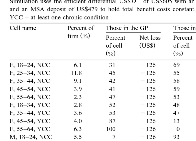
Table 3 shows the pattern of distribution of gains and losses when the employer benefit cost is held constant. Those who lose the most are older workers with
Ž
chronic conditions while the gain relative to the initial situation with everyone in
.
the GP is obtained primarily by male workers without chronic conditions,
Table 2
The efficient premium differential with varying allocations between the employer and its employees The efficient differential US$ D) of US$605 causes 39% to remain in the generous plan and 61% to
enroll in the MSArCHP.
Allocation of differential Compensation costs Net gain
GP MSA Total Wage All Those in Those
a
premium deposit benefits offset workers the GP in the
costs MSArCHP
0 605 1811 y126 148 0 241
126 479 1685 0 22 y126 115
148 457 1663 22 0 y148 93
241 364 1570 115 y93 y241 0
605 0 1206 479 y457 y605 y364
a
Table 3
Simulation results using efficient premium differential: distribution of employees’ gains and losses by risk type
Simulation uses the efficient differential US$ D) of US$605 with an employee premium of US$126
and an MSA deposit of US$479 to hold total benefit costs constant. NCCsno chronic conditions. YCCsat least one chronic condition
Cell name Percent of Those in the GP Those in the MSArCHP All workers
Ž .
firm % Percent Net loss Percent Net Net
Ž .
of cell US$ of cell gain gain
Ž .% Ž .% ŽUS$. ŽUS$.
F, 18–24, NCC 6.1 31 y126 69 55 y1
F, 25–34, NCC 11.8 45 y126 55 27 y41
F, 35–44, NCC 9.1 42 y126 58 29 y36
F, 45–54, NCC 3.9 41 y126 59 35 y31
F, 55–64, NCC 2.3 47 y126 53 21 y48
F, 18–34, YCC 2.8 52 y126 48 y47 y88
F, 35–44, YCC 3.6 53 y126 47 y58 y94
F, 45–54, YCC 4.0 87 y126 13 y124 y126
F, 55–64, YCC 6.3 100 y126 0 nra y126
M, 18–24, NCC 5.5 7 y126 93 220 196
M, 25–34, NCC 12.3 7 y126 93 216 193
M, 35–44, NCC 9.9 7 y126 93 224 201
M, 45–54, NCC 5.1 20 y126 80 103 57
M, 55–64, NCC 2.9 34 y126 66 63 y1
M, 18–34, YCC 2.5 16 y126 84 130 90
M, 35–44, YCC 3.7 26 y126 74 69 18
M, 45–54, YCC 3.6 50 y126 50 y12 y69
M, 55–64, YCC 4.6 100 y126 0 nra y126
ENTIRE 100 39 y126 61 115 22
although, among female workers without chronic conditions, more than half are better off by choosing the MSA.6
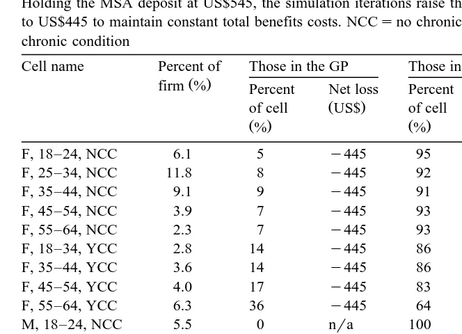
We simulate the option of a fixed dollar contribution toward each plan by assuming that the initial MSA deposit equals the average savings if everyone chose the MSArCHP option. We then incrementally raise the GP employee premium to maintain the original level of benefits costs; the results from this iteration are shown in Table 4. In this case, high risks are made worse off, and conventional coverage goes into a ‘‘near-death’’ spiral, falling to an 8% share. At
6
Table 4
Simulation results using inefficient fixed dollar contribution: distribution of employees’ gains and losses by risk type
Holding the MSA deposit at US$545, the simulation iterations raise the employee premium of the GP to US$445 to maintain constant total benefits costs. NCCsno chronic conditions. YCCsat least one chronic condition
Cell name Percent of Those in the GP Those in the MSArCHP All workers
Ž .
firm % Percent Net loss Percent Net Net
Ž .
of cell US$ of cell gain gain
Ž .% Ž .% ŽUS$. ŽUS$.
this point, the gain from offering the MSArCHP option is still positive, at US$10, but less than the efficient outcome. Moreover, there exists a larger dispersion of net gains across employee types.
Compared to the fixed dollar premium, implementation of the efficient
pre-Ž .
mium differential increases aggregate welfare as in the numerical example . However, in this case, a strategy of holding employer payroll cost constant will reduce the welfare of high risks, relative to the ‘‘GP-only’’ situation; there is no way to introduce the MSArCHP in a Pareto fashion, in contrast to the two-risk-class case. The reason is that, with multiple risk two-risk-classes, a payment differential equal to the additional cost of the GP for the marginal risk class will not cover the
Ž .
additional cost of that plan for the aÕerage persons at yet higher levels of risk
who will choose it. Wages therefore will have to fall, and the high risks made
Ž
worse off. However, even those high risks that lose will lose less by choosing the
. Ž .
costs to high risks significantly. The reason is that, on average, the GP is not very much more efficient for high risks than is the CHP.
4. Employer motivation
While the analysis thus far shows that there exists an employer-set premium differential that could keep total labor costs unchanged and lead to an efficient allocation of workers to plans, it provides no obvious basis for concluding that employers will choose this differential. At the simplest level, if employers for some reason wished to prevent any redistribution against high risks, they would choose not to offer the MSArCHP option even though it is efficient for some. If employers wished to offer MSAs but not make high-risks worse off, employers
Ž .
could follow the inefficient rule, as suggested by Thorpe 1995 , of adjusting the MSA contribution downward so total net payments for each plan equaled that
Ž .
plan’s enrollees’ original cost in the GP. Simulation results not shown indicate that 21% of workers — only younger males with no chronic conditions — would take the MSArCHP as the MSA deposit falls to US$268, and the net gain per worker falls to US$11. If, in contrast, employers wished to offer advantage to low risks, they might choose the efficient plans, the fixed dollar contribution, or might just go straight to offering the MSArCHP option only.
If the employer was concerned with maximizing the total welfare of all employees, one of the efficient plans might be chosen. However, what if the employer was only concerned with minimizing total labor costs and the supply of workers of both risk types responded to the total value of compensation received? Given the assumption of equal productivity and equal money wages in the initial situation, encouraging high-risk workers to self-identify and self-select might appear to be a reasonable strategy. Raising premiums for the generous coverage is a no-lose strategy. If high risks pay those higher premiums, net labor costs are reduced. If they react by moving away, and are replaced by low risk workers attracted by the MSArCHP plan, labor costs are reduced. We conjecture that the premium differential against the high risks can profitably be increased beyond the efficient level if the supply elasticity is the same for all risk types; it will be profitable to continue to push up the premium until all high risks are driven away unless the risk differential is small andror the high risk labor supply is highly elastic.
5. Conclusion
employer contribution approach. By definition, the efficient strategy avoids death
Ž .
spirals except when it is efficient for all employees to be in one plan , and maximizes the average net benefit per employee. Compared to some initial starting points, however, implementing the efficient strategy may make some risk groups worse off. High risks may be made worse off if the initial starting point is a single GP, whereas low risks could be made worse off in moving to the efficient plan from the near-death-spiral, CHP-only, option.
In the specific simulation of adding an MSArCHP option for a workforce that typifies insured adults, these general conclusions are illustrated. Compared to a single GP, offering an MSArCHP option with fixed employer contributions leads to significant reductions in well being of some high risk groups, and barely leads to a positive gain overall. Implementing the efficient plan instead increases the average gain, and reduces the average loss of those who lose to a modest amount. The simulation results also show, however, that even in the best of circumstances, the average welfare gain from adding the MSArCHP option is moderate relative to total medical care spending, although the pure cost containment effect is more substantial. Conversely, however, the consequences for high risks of adding the new plan in an efficient fashion, while negative, are also minimal. These effects seem small relative to the political controversy associated with this option.
While it is risky to generalize from these simulations, they do suggest that the absolute gains from adding the MSArCHP option to the employer are likely to be relatively small. If the employer wanted to avoid the controversy associated with risk segmentation, such plans might therefore be unattractive. However, if the employer wanted to appeal to the low risk segment of the workforce, perhaps because its supply is more responsive to compensation, adding such a plan would target that segment.
Acknowledgements
This research was supported by the Robert Wood Johnson Foundation’s Grant a31351. We are grateful for the helpful comments from discussant Richard Zeckhauser and other participants of NBER’s Insurance Project Meeting at Cambridge in February, 1999. We also appreciate comments from David Cutler, Joseph Newhouse, and two anonymous referees.
References
American Academy of Actuaries, 1995. Medical savings accounts: cost implications and design issues. AAA Public Policy Monograph.
Burman, L., 1997. Medical savings accounts and adverse selection. Urban Institute Mimeo.
Cutler, D., Reber, S., 1998. Paying for health insurance: the tradeoff between competition and adverse
Ž .
selection. Quarterly Journal of Economics 113 2 , 433–466.
Cutler, D., Zeckhauser, R., 1997. Adverse selection in health insurance. NBER Working Papera6107.
Ž .
Goldstein, G., Pauly, M., 1976. Group health insurance as a local public good. In: Rosett, R. Ed. , The Role of Health Insurance in the Health Services Sector. NBER, Cambridge.
Health Care Financing Administration, Office of the Actuary, 1997. National health expenditures,
Ž .
1996. Health Care Financing Review 19 1 , 161–200.
Nichols, L. et al., 1996. Tax-Preferred Medical Savings Accounts and Catastrophic Health Insurance Plans: a Numerical Analysis of Winners and Losers. Urban Institute Mimeo.
Pauly, M., 1974. Overinsurance and public provision of insurance: the roles of moral hazard and
Ž .
adverse selection. Quarterly Journal of Economics 88 1 , 44–62.
Pauly, M., 1997. Health Benefits at Work: an Economic and Political Analysis of Employment-based Health Insurance. University of Michigan Press, Ann Arbor.
Rothschild, M., Stiglitz, J., 1976. Equilibrium in competitive insurance markets: an essay on the
Ž .
economics of imperfect information. Quarterly Journal of Economics 90 4 , 630–649.
Ž .
Thorpe, K., 1995. Medical savings accounts: design and policy issues. Health Affairs 14 3 , 254–259. Zabinski, D. et al., 1999. Medical savings accounts: microsimulation results from a model with adverse
Ž .