Performance Evaluation of Ordinary Kriging and Inverse Distance Weighting Methods for Nickel Laterite Resources Estimation Waterman Sulistyana Bargawa and Hendro Purnomo
Master of Mining Engineering, UPN “Veteran” Yogyakarta, 55283 SWK 104 Yogyakarta, Indonesia
AbstractThe choice of an accurate interpolation technique for predicting nickel grade and other elements in unsampled location is an important issue in mineral resources estimations. The use of kriging variance on geostatistics method for measuring of confidence level is difficultto apply directly. This study introduces the use of RMSE (root mean square error) in the selection of the best variogram model related to the accuracy of the estimation performance. In this study, use OK (ordinary kriging) and IDW (inverse distance weighting) techniques for nickel laterite resource estimation. Result indicates at low CV values, OK model is relatively more accurate than IDW that is shown by a low RMSE value.Correlation between skewness and IDW techniques indicates that data with low skewness (<1)IDW with a power of1 is better thanother power value and data with high skewness (>2.5) a power of 2 yielded the most accurate estimates.
Keywords: geostatistics, nickel laterite, RMSE.
AbstrakPemilihan teknik interpolasi yang akurat untuk memprediksi kadar nikel dan unsurlain di lokasi yang tidak memiliki data merupakan masalah penting dalam penaksiran sumberdaya mineral. Penaksiran sering mengabaikan nilai parameter statistik dasaryaitu CV (koefisien variansi) dan skewness yang berhubungan dengan teknik interpolasi yang dipilih. Penggunaan variansi kriging pada metode geostatistik ternyata sulit dipakai secara langsung untuk mengukur tingkat keyakinan taksiran kadar. Penelitian ini mengenalkan penggunaan RMSE (root mean square error) dalam pemilihan model variogram yang berkaitan dengan akurasi kinerja teknik penaksiran. Teknik penaksir OK (ordinary kriging) dan IDW (inverse distance weighting) dipakai untuk studi kasus estimasi sumberdaya nikel. Pada nilai CV rendah, model OK relatif lebih akurat dibandingkan dengan model IDW yang ditunjukkan dengan nilai RMSE yang rendah. Data dengan nilai skewness rendah, model IDW pangkat 1 lebih akurat dibandingkan dengan nilai pangkat yang lain, sedangkan pada nilai skewness yang besar, model IDW pangkat 2 menghasilkan penaksiran lebih akurat.
Kata kunci : geostatistik, laterit nikel, RMSE.
1. Introduction
There are several interpolation method was developed by using computer tool can be used to estimate the potential resources and reserves, among other are IDW and OK method. In the process IDW is simpler and quicker unlike kriging that requires preliminary modeling step of the relationship between a variance and distance [1]. The IDW method has been applied mainly because of simple and quick while kriging has been used due to provides best linear unbiased estimates [2]. As a comparison the IDW and OK procedure were applied to evaluate laterite nickel resources in this research. Nickel laterite is product of intensive deep weathering of olivine rich ultramafic rocks and their serpentinized equivalents. In general profile of the nickel laterite can be divided into limonite zone, saprolite zone and bed rock [3, 4].
The research area is located in East Halmahera regency, North Maluku Province of Indonesia which is a region nickeldeposit well developed (Figure 1). Geologically the area (see Figure 2) is located in east arm of Halmahera that is widely occupied by ultrabasic rocks complex, as a resource potential of nickel laterite, with predominant north-east and north – northnorth-east trending structure [5].
Objective of the research was to evaluate the relative performance of the IDW and OK in predicting amount of nickel, based on root mean square error (RMSE) value, and to analyze the relationship between statistic parameters and performance of the methods.
2.Methods and Material
Kriging is spatial prediction technique for linear optimum unbiased interpolation with a minimum
International Conference on Science and Technology 2nd
mean interpolation error [6]. This method work with the parameter obtained from the result of fitting between semivariogram experimental and theoretical model as main base [7]. The most widely used models are spherical, exponential and Gaussian [8]. In this study to select a semivariogram theoretical model is based on the root mean square error (RMSE) value whereas the smallest value was chosen as the best model [9]
A semivariogram experimental defined by equation below [8].
ɣ
(
h
)=
1
2
n
(
h
)
∑
i=1 n(h)
[
Z
(
x1
)
−
Z
(
x
i+h)
]
2 (1)where:
Z
(
x
i)
: Sample value of the variable at pointx
iZ
(
x
i+
h
)
: Sample value of the variable at apoint distance h from point
x
i .ɣ
(
h
)
: The experimental semivariogram value at the distance interval h.n
(
h
)
: Number of sample pairs within the distance interval h.Ordinary kriging (OK) is one of the basic on kriging methods that provides an estimate at unobserved location, based on weighted average of around observed sites within an area [1]. Some points that it should be noted in OK prediction are [10]:
OK prediction at an unsampled location
Z
^
is defined by an equation:^
Z
=
∑
¿1 n
λ
i. Z
i (2)The weight
λ
i calculated by a formula:∑
i n
λ
i. C
(
i , j
)+
µ
=
C
(
i ,
0
)
, with
∑
i=1 n
λ
i=
1
(3)
Kriging variance can be expressed with the following equation:
λ
iC
i0∑
i=1 n
¿
+
µ
(
¿¿
)
σ
R2
=
C
(
0
)−
¿
(4)
where:
Z
i : A sample value at point i.C
(
i , j
)
: Covariance between sample i andsample j.
µ : Lagrange multiplier.
C
(
i ,
0
)
: Covariance between sample andblock0.
To identify a sample weight, IDW assumed that degree of correlations and similarities between neighbors is proportional to the distance between them [1]. The IDW equation that is used in weighting is written below [8]
w
i=
1
di
k∑
i=1 n
1
di
k(5)
To estimate a predicted point is used equation below:
^
Z
0=
∑
i=1 n
w
i. Z
i (6)where:
^
Z
0 : Target points where the value should beestimated.
w
i : A sample weight in point i.d
i : A distance between point i and a prediction point.k
: A power parameter.Z
i : A sample value in point i.Putu Indra Christiawan
THE SPATIAL PATTERNS
Figure 1: Location of The Research Area in Halmahera Indonesia
Figure 2. Regional Geological Map of East Halmahera Indonesia
To compare the accuracy of interpolation method was used parameter of root mean square error (RMSE). The RMSE indicated deviate from the measured value and it is calculated with equation [1]:
RMSE
=
√
1
n
∑
i=1n
(
Z
^
(
x
i
)
−
Z
(
x
i)
)
2(7)
where:
^
Z
(
x
i)
: The estimation value.Z
(
x
i)
: The observed value.n : Total number of the estimation.
The prediction is not much deviate if a root mean square error value is low.
3. Result and Discussion
Geochemical assay data, consisted of Ni, Fe, Co, MgO, and thickness used in this research were obtained from 266holes of core drilling. The assay data then discriminated and composited into two zone namely: limonite and saprolite base on the Fe content, where Fe >25% implied in limonite zone and Fe ≤25% included in saprolite zone. Summary statistic for all variables obtained from 266 composite data in saprolite zone and 256 data in limonite zone are given in Table 1.
Table 1. Descriptive Statistics for Saprolite and Limonite Zone
Zone Variable CV Mean Minimum Maximum Standard
deviation Skewness Kurtosis
Saprolite Ni 0.25 1.44 0.57 2.47 0.36 0.16 2.71
MgO 0.55 19.65 0.02 83.50 10.90 2.67 17.62
Thickness 0.53 11.94 1.70 31.00 6.13 0.74 2.92
Limonite
Ni 0.11 1.27 0.91 1.61 0.14 -0.19 2.56
Fe 0.14 34.34 19.95 46.08 4.66 -0.41 3.25
Co 0.19 0.10 0.01 0.19 0.019 0.14 7.71
MgO 0.87 4.94 0.01 42.03 4.34 6.00 48.43
Thickness 0.49 14.33 3.00 32.00 7.09 0.28 2.23
To identify the possible spatial structure of different variables, semivariogram experimental were calculated according to anisotropy model.Assigning the best semivariogram model for each variable was based on root mean square error (RMSE) value, whereas the lowest RMSE value was chosen as the best model [9].
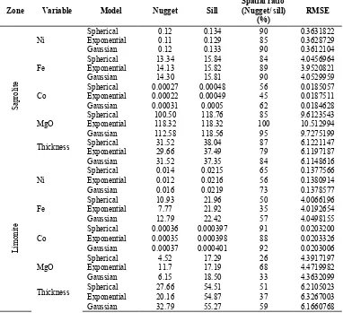
Table 2 present the RMSE value and different theoretical semivariogram models as a result of matching with experimental semivariogram for each variable. Among different theoretical model were tested, the gaussian model were identified as the best fit in most variable and the spherical model
as the most second. In case of Fe in saprolite zone, the best spatial variation was described by the exponential model. Parameters from the best of the theoretical semivariogram model were then used in estimation process by method of ordinary kriging (OK). In this study estimation process by IDW utilizes semivariogram and anisotropic ellipsoid parameter as well. IDW predictions were also exercised by varying number of power, from 1 to 3, and used a number of the closest neighboring points range from 3 to 20 equal with were used in the kriging process. Result of the RMSE according to OK and IDW power of 1, 2 and 3 were given in Table 3 and Table 4.
Table 2. The Fitted Semivariogram Models, Their Parameters and The RMSE Result
Zone Variable Model Nugget Sill
Spatial ratio (Nugget/ sill)
(%)
RMSE
S
apr
ol
it
e
Ni
Spherical 0.12 0.134 90 0.3631822
Exponential 0.11 0.129 85 0.3628729
Gaussian 0.12 0.133 90 0.3612104
Fe
Spherical 13.34 15.84 84 4.0456964
Exponential 14.13 15.82 89 3.9520821
Gaussian 14.30 15.81 90 4.0529959
Co
Spherical 0.00027 0.00048 56 0.0185057
Exponential 0.00022 0.00049 45 0.0187511
Gaussian 0.00031 0.0005 62 0.0184628
MgO
Spherical 100.50 118.76 85 9.6123543
Exponential 118.32 118.32 100 10.512994
Gaussian 112.58 118.56 95 9.7275199
Thickness Spherical 31.52 38.04 87 6.1221147
Exponential 29.66 37.49 79 6.1197187
Gaussian 31.52 37.35 84 6.1148616
L
im
oni
te
Ni
Spherical 0.014 0.0215 65 0.1377566
Exponential 0.012 0.0216 56 0.1380914
Gaussian 0.016 0.0219 73 0.1378577
Fe
Spherical 10.93 21.96 50 4.0066196
Exponential 7.77 21.92 35 4.0192654
Gaussian 12.79 22.42 57 4.0498155
Co
Spherical 0.00036 0.000397 91 0.0203200
Exponential 0.00035 0.000398 88 0.0203326
Gaussian 0.00037 0.000401 92 0.0203006
MgO
Spherical 4.52 17.29 26 4.3917197
Exponential 11.7 17.19 68 4.4719982
Gaussian 6.15 18.50 33 4.3632099
Thickness Spherical 27.66 54.51 51 6.2105023
Exponential 20.16 54.87 37 6.3267003
Gaussian 32.79 55.27 59 6.1660768
Table 3. Result of The RMSE According to OK and IDW Powers Of 1-3 for Saprolite Zone
Zone Variable Skewness
Spatial ratio (Nugget/ sill)
(%)
Interpolation
model RMSE
Saprolite Ni 0.16 90 OK-Gaussian 0.361210
IDW 1 0.389315
IDW 2 0.389915
Putu Indra Christiawan
THE SPATIAL PATTERNS
IDW 3 0.392149
Fe 0.66 89
OK-Exponential 3.952082
IDW 1 4.017983
IDW 2 4.073498
IDW 3 4.228154
Co 0.17 56
OK-Gaussian 0.018463
IDW 1 0.018515
IDW 2 0.018815
IDW 3 0.019268
MgO 2.67 85
OK-Spherical 9.612354
IDW 1 9.638006
IDW 2 9.606666
IDW 3 9.781412
Thickness 0.74 84
OK-Gaussian 6.114862
IDW 1 6.076767
IDW 2 6.159322
IDW 3 6.319711
Table 4. Result of The RMSE According to OK and IDW Powers of 1-3 for Limonite Zone
Different classes of spatial dependence for both saprolite and limonite variables were evaluated by the ratio between the nugget variance and sill value [11]. Based on Table 3 and Table 4, the best fitted semivariogram analysis for all variables indicated nugget/sill equal to 33-92% which was classified as medium to weak spatial dependence. Result of the IDW prediction with using different power value, indicated that IDW with power of 2 provided the most accurate prediction if the data had skewness
>2.5, whereas data with skewness value <1 the best estimation was yielded by IDW with power of 1. Table 3 and Table 4 shows parameters of skewness and result of RMSE. Table 5 suggested that there was a relationship between value of CV and RMSE, while the data set had CV value <0.5 then result of the OK prediction was better than IDW and if value of CV >0.5, so the IDW prediction more accurate than OK.
Table 5. Parameters of Coefficient of Variation (CV), Skewness and Result of RMSE
Variable Zone CV Skewness Interpolation
model RMSE
Ni
Saprolite 0.252 0.16 OK-Gaussian 0.361210
IDW 1 0.389315
Limonite 0.113 -0.19 OK-Spherical 0.137757
IDW 1 0.149785
Fe
Saprolite 0.29 0.66 OK-Exponential 3.952082
IDW 1 4.017983
Limonite 0.136 -0.41 OK-Spherical 4.006620
IDW 1 4.143441
Co
Saprolite 0.41 0.17 OK-Gaussian 0.018463
IDW 1 0.018515
Limonite 0.188 -0.14 OK-Gaussian 0.020301
IDW 1 0.021336
MgO
Saprolite 0.55 2.67 OK-Spherical 9.612354
IDW 2 9.606666
Limonite 0.87 6 OK-Gaussian 4.363210
IDW 2 4.356661
Thickness
Saprolite 0.53 0.74 OK-Gaussian 6.114862
IDW 1 6.076767
Limonite 0.49 0.28 OK-Gaussian 6.166077
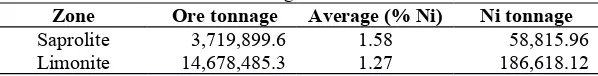
Estimation of nickel deposit was based on the two dimensional model with the result was stated by tonnage. The tonnage was obtained from the result of between volume times density of each zone, while the volume was obtained from the result of between thickness of each zone by square of the drill hole grid (50 x 50 m). In this research was assumed the density of the limonite was 1.6 ton/m³ and the saprolite was 1.5 ton/m³ with cutoff grade value were 1.5% and 1 % for the saprolite and
limonite ore respectively. Base on the best performance interpolation method was chosen, the amount of the nickel resources in the saprolite zone was calculated with using OK-Gaussian procedure for Ni variable and IDW power of 1 technique for variable of thickness, while nickel in the limonite zone was calculated according to OK-Spherical and Gaussian procedures for both Ni and thickness variables respectively. Result of the nickel resources estimation was presented in Table 6.
Table 6. Tonnage of Ni Resources
Zone Ore tonnage Average (% Ni) Ni tonnage
Saprolite 3,719,899.6 1.58 58,815.96
Limonite 14,678,485.3 1.27 186,618.12
5.Conclusion
Based on the discussion above, some conclusions can be noted:
a) In the saprolite zone, performance of the OK procedure was relatively better than IDW for the Ni variable otherwise for the thickness variable performance of the IDW power of 1 was better than OK. In the limonite zone, the OK technique has better performances than IDW for both variable of Ni and thickness. b) The Ok procedure has better performance than
IDW when the data set has coefficient of variation <0.5 whereas the IDW procedure produce better performance than OK when the data set has CV >0.5.
c) The IDW power of 2 has better prediction than IDW with other power value for if the data set has high skewness value (>2.5) otherwise IDW with power of 1 resulted in better estimation if the data with low skewness (<1).
d) Based on the best performance of the interpolation method the nickel resources estimation in the study area was estimated by using OK procedure for Ni variable and IDW power of 1 for thickness variable in the saprolite zone, while in the limonite zone was used OK procedure for both Ni and thickness variables.
References
1. Yasrebi, J., Saffari, M., Fathi, H., Karimian, N., Moazallahi, M., & Gazni, R. (2009). Evaluation and comparison of ordinary kriging and inverse distance weighting methods for prediction of spatial variability of some soil chemical parameters. Research Journal of Biological Sciences, 4(1), 93-102.
2. Almasi, A., Jalalian, A., & Toomanian, N. (2014). Using OK and IDWmethods for prediction thespatial variability of a horizon depth and OM in soils of Shahrekord, Iran.
Agrochimica, 58(1).
3. Butt, C. R., & Cluzel, D. (2013). Nickel laterite ore deposits: weathered serpentinites.
Elements, 9(2), 123-128.
4. Elias, M. (2002). Nickel laterite deposits-geological overview, resources and exploitation. Giant ore deposits: Characteristics, genesis and exploration. CODES Special Publication, 4, 205-220.
5. Apandi, T., & Sudana, D. (1980). Geologic map of the Ternate quadrangle, North Maluku.
Geological Research and Development Centre, Bandung, Indonesia.
6. Mousavifazl, H., Alizadh, A., & Ghahraman, B. (2013). Application of Geostatistical Methods for determining nitrate concentrations in Groundwater (case study of Mashhad plain,
Iran). International Journal of Agriculture and Crop Sciences, 5(4), 318.
7. Bargawa, W. S., & Amri, N. A. (2016, February). Mineral resources estimation based on block modeling. In Progress in AppliedMathematics in Science and Engineering Proceedings (Vol. 1705, p. 020001). AIP Publishing.
8. Isaaks, E. H. (1989). Applied geostatistics (No. 551.72 I86). Oxford University Press.
9. Suryani, S., Sibaroni, Y., & Heriawan, M. N. (2016). Spatial Analysis 3d Geology Nickel Using Ordinary Kriging Method. Jurnal Teknologi, 78(5).
10. Armstrong, M. (1998). Basic linear geostatistics. Springer Science & Business Media.
11. Cambardella, C. A., Moorman, T. B., Parkin,
T. B., Karlen, D. L., Novak, J. M., Turco, R. F., & Konopka, A. E. (1994). Field-scale variability of soil properties in Central Iowa.